PID Controller & Loops: A Comprehensive Guide to Understanding and Implementation
This guide delves into the basics and components of PID control, implementation, application examples, impacts, challenges, and solutions aiming to provide readers with a thorough understanding of this integral concept.

21 Jun, 2023. 18 minutes read
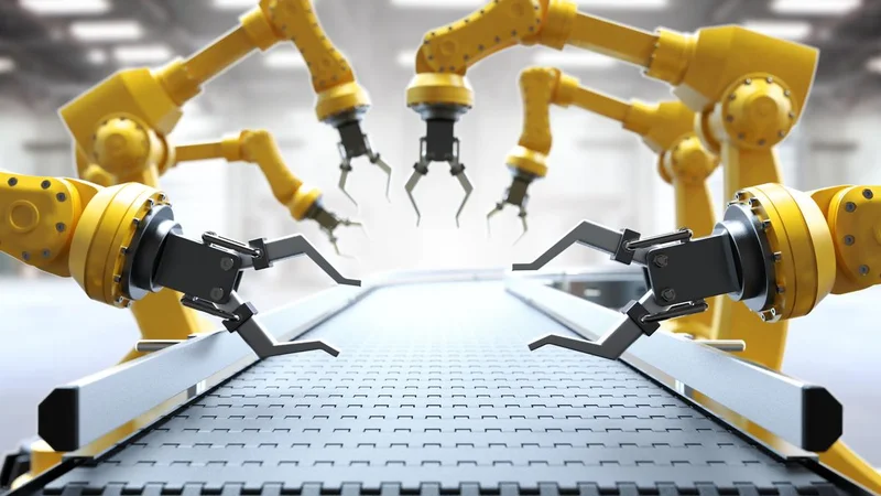
Robotic arms in the industry based on PID loop
Introduction
A Proportional-Integral-Derivative (PID) controller or PID loop is vital to industrial control systems. It is a robust control mechanism that manipulates an input variable based on the error signal: the difference between the target value (setpoint) and the measured value (process variable). PID loop involves three parameters: the Proportional, the Integral, and Derivative values. The PID loop alters its output to reach the desired setpoint with minimum error and optimal speed, making it an essential tool in various engineering and technological applications.
Basics of PID Control
The PID controller algorithm centers around a feedback control loop mechanism. [1] When a PID loop is in action, it calculates an 'error' value as the difference between a measured process variable and a desired setpoint. The controller then seeks to minimize this error over time by adjusting control variables.
The term PID represents Proportional, Integral, and Derivative. These correspond to three different mathematical computations applied to the error signal to drive the controller's output. The proportional term produces an output value proportional to the current error value. The integral term is proportional to both the magnitude of the error and the duration of the error, making it crucial for long-term accuracy. The derivative term is computed based on the rate of change of the error, providing a prediction of future error based on the current rate of change.
As a robust control mechanism, the PID controller is suitable for systems where the mathematical model is unavailable or too complex to be modeled. In such cases, the PID controller, with its tuning parameters, can ensure the desired level of performance.
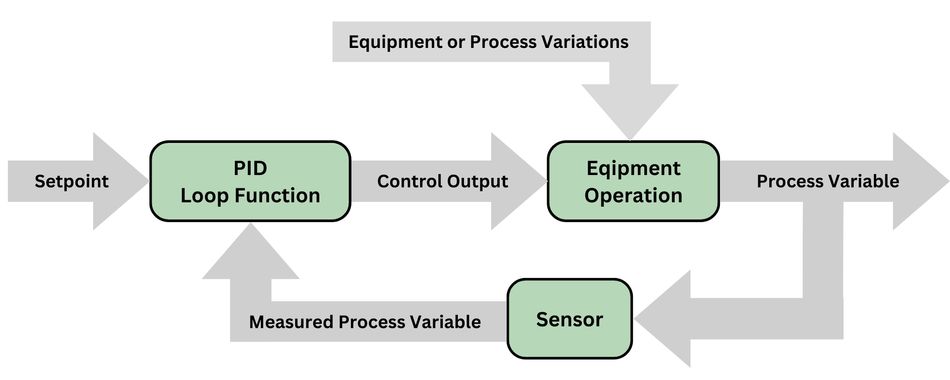
Concept of Feedback Control
Feedback control is a system that uses information from measurements to manipulate a variable to achieve the desired result. The output is fed back into the input, thereby closing the loop. By continually checking the output and adjusting the input accordingly, the system self-regulates to maintain the desired output.
In a PID loop, the measured process variable, such as temperature or velocity, is continually fed back and compared with the desired setpoint. The difference between the setpoint and the measured value is calculated as an error. The PID controller works to minimize this error by adjusting the control variable, such as the power applied to a heater or the position of a valve.
The essence of feedback control lies in its ability to use the output data to influence the input, ensuring the system's response aligns with the desired setpoint. This feature lends the system its self-regulating characteristic, making it resilient to external disturbances and variations in system dynamics.
PID and PI control are both types of feedback control systems that use the proportional, integral, and derivative terms of the error signal to calculate the control output. The main difference between PI and PID control is that PID control includes the derivative term, while PI control does not. However, PI control can sometimes be unstable, especially in systems with fast dynamics.
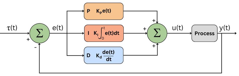
The PID Algorithm
The PID algorithm uses three separate modes to calculate the output that will be applied to the control variable. [2]
The first mode is the Proportional or P mode. The controller output is directly proportional to the current error value in P mode. This error differs between the desired setpoint and the measured process variable. Mathematically, the proportional term is expressed as:
Pout = Kp * e(t), where Pout is the proportional output, Kp is the proportional gain, and e(t) is the instantaneous error at the time 't'.
The second mode is the Integral or I mode. PID controller's integral part considers the magnitude of the error and the duration for which it persists. It is designed to respond to accumulated errors over time, contributing to the elimination of the residual steady-state error that occurs with a P-only controller. The mathematical representation of the integral term is:
Iout = Ki ∫ e(t) dt, where Iout is the integral output, Ki is the integral gain, and the integral of e(t) is over the time from the start to the current instant.
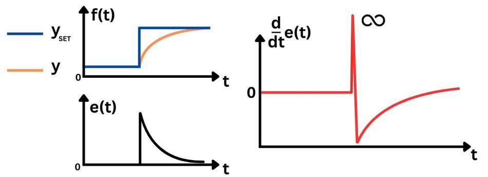
The third mode is the Derivative or D mode. The derivative part of the PID controller is concerned with the rate of change of the error. It provides a prediction of future errors based on the current rate of change and helps reduce overshoot and settling time. The derivative mode can increase the rise time of the system, especially if the derivative time constant is too large. It can be represented as:
Dout = Kd * de(t)/dt, where Dout is the derivative output, Kd is the derivative gain, and de(t)/dt is the rate of change of error with respect to time.
The overall PID output is a weighted sum of these three terms and can be represented as:
PIDout = Pout + Iout + Dout.
This combined output is then used to adjust the control variable, seeking to minimize the error, and making the system respond optimally to changes in the setpoint or any disturbances.
Components of PID Control
PID control is structured around three distinct elements, each contributing to the overall control mechanism. These components are the Proportional, Integral, and Derivative terms. They are combined to regulate the process variable, each addressing a specific aspect of the control process.
The Proportional Term
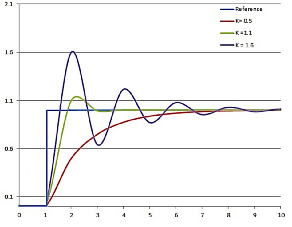
The Proportional term (P) forms the foundation of PID control. It provides an output value, directly proportional to the current error signal. The error signal is the difference between the desired setpoint and the current measurement of the process variable. This term alone can manage control, but with some level of steady-state error, as it depends on the present error only. The proportionality constant, also known as the controller's gain, adjusts the controller's responsiveness. A high gain results in a large change in output for a given change in error, making the system more responsive to changes in the setpoint or load, but it may also lead to system instability.
The proportional term's effectiveness lies in its immediate response. It reacts promptly to changes in the error signal, enabling a fast system response. However, it's essential to balance the speed of response with system stability. Too large a gain can cause the system to oscillate, while too small a gain may result in sluggish performance. Therefore, tuning the proportional gain is critical to achieving a desirable trade-off between system responsiveness and stability.
The proportional term's output is mathematically represented as:
Pout = Kp * e(t), where Kp denotes the proportional gain and e(t) is the instantaneous error.
The effect of this term is most prominent when a sudden change in the setpoint occurs. This causes an immediate change in the controller output proportional to the magnitude of the change.
The Integral Term
In the PID control system, the Integral term (I) complements the Proportional term by addressing its shortcomings. Specifically, the integral term mitigates the steady-state error associated with a Proportional control system. Steady-state error is the absolute difference between the process variable and the setpoint once the system has settled following a disturbance or change in the setpoint.
The Integral term accomplishes this by accumulating past error signals over time and applying a correction based on their cumulative value. In essence, it integrates the error over time. The longer the error persists, the larger the integral term becomes. This effect allows the controller to apply an increasing corrective action, thus reducing the steady-state error. However, this can sometimes result in an overshoot due to the Integral term's cumulative nature, which then requires the corrective action of the Derivative term.
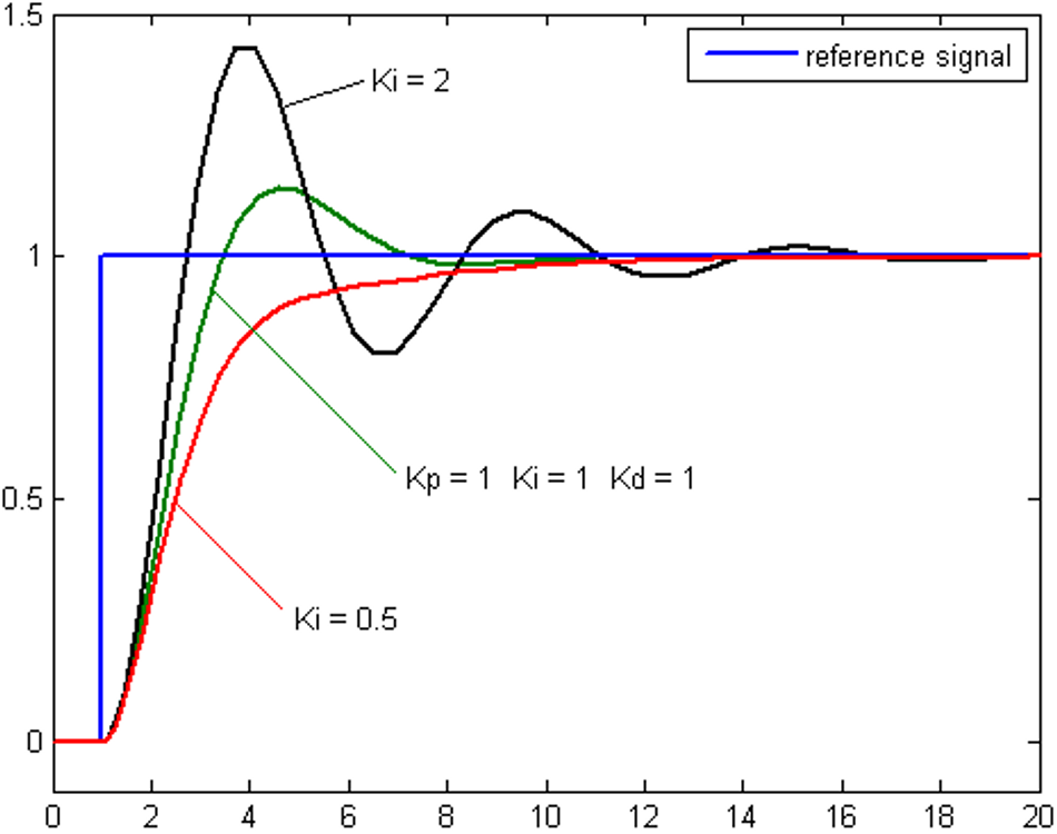
Mathematically, the output of the integral term is calculated as:
Iout = Ki * ∫ e(t) dt, where Ki is the integral gain, e(t) is the instantaneous error, and the integral is calculated over time.
Here, Ki determines the rate at which the integral action takes effect. A high Ki results in a fast response to accumulated errors, while a low Ki causes a slower response.
Tuning the integral gain (Ki) is critical in achieving the right balance in the controller's response. A large Ki might lead to system instability by causing oscillations, while a small Ki might result in a sluggish response to steady-state errors. Therefore, the right Ki value is vital for a smooth and stable system response that adequately compensates for steady-state errors.
The Derivative Term
The Derivative term (D) in a PID controller aims to predict the future behavior of the error by evaluating its rate of change. This feature makes it a vital element in the PID controller. While the Proportional term reacts to the present error and the Integral term addresses past errors, the Derivative term considers the future trends of the error. This is vital to dampen the system's response and avoid overshooting the setpoint.
The rate of change in error is simply the derivative of the error with respect to time. When errors rapidly change, the Derivative term responds by applying a strong corrective action. Conversely, when the error changes slowly or remains constant, the corrective action from the Derivative term is reduced.
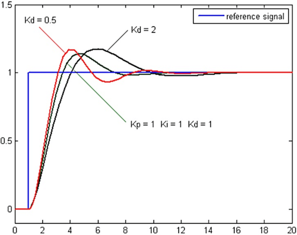
The mathematical expression for the Derivative term is:
Dout = Kd * (de/dt) where Kd is the derivative gain and de/dt is the rate of change of error.
The derivative gain, Kd, determines the influence of the Derivative term on the overall control action. A larger Kd means a larger damping effect, reducing overshoot but potentially leading to a slower response. Conversely, a smaller Kd results in a faster response but with a risk of overshooting.
Tuning the Derivative term can be tough. While it is valuable in controlling rapid changes, it can also amplify high-frequency noise in the error signal. A proper balance is crucial to preventing excessive noise while maintaining the system's quick and accurate response to changes.
Automated PID Tuning
Automated PID tuning is a method that aims to automatically find the optimal tuning parameters for a PID controller. This can be a preferable alternative to manual tuning, which is often time-consuming and requires a fair amount of expertise. Automated PID tuning methods rely on algorithms that iteratively adjust the PID controller's tuning parameters, which are the Proportional gain (Kp), the Integral time constant (Ti), and the Derivative time constant (Td).
The algorithms seek to minimize the error between the setpoint and the process variable. By continuously adjusting the parameters, the PID controller adapts to changes in the process, which can be unpredictable and nonlinear. Automated tuning handles these changes by continually optimizing the PID parameters, maintaining control quality even under varying operating conditions.
Ziegler-Nichols method and the relay feedback test are widely used methods for automated PID tuning. The Ziegler-Nichols method uses the process's ultimate gain and period of oscillation at this gain to set the PID parameters. [3] In contrast, the relay feedback test introduces a square wave signal into the system and analyzes the system's output to derive PID parameters.
However, automated PID tuning is not a one-size-fits-all solution. The tuning parameters derived from automated tuning methods may not be optimal for all operating conditions or all types of processes. Hence, manual fine-tuning may still be required to ensure optimal performance for specific applications. However, automated PID tuning can significantly reduce the time and expertise required for the initial setup and ongoing adjustments of the PID controller.
Implementing PID Control
A PID loop can be implemented in various systems, ranging from mechanical systems like automobile cruise control to complex process control applications. In implementing a PID controller, the key challenges are selecting appropriate values for the proportional, integral, and derivative gains and ensuring the stability of the closed loop control.
The proportional, integral, and derivative controller gains are tunable parameters of a PID controller that must be adjusted carefully to achieve optimal performance. The chosen values will directly affect how the system responds to changes in the setpoint or disturbances, determining the speed of the response, the extent of overshoot, and the stability of the system. Therefore, proper tuning of these gains is crucial in PID control.
Recommended Reading: Understanding Process Control: An important technique for industrial processes
Tuning a PID Loop
The process of determining the optimal gains for a PID controller is known as tuning. Several PID tuning methods generally involve iterative trial-and-error procedures or analytical methods based on the mathematical model of the system.
The most common tuning method is the Ziegler-Nichols method, which provides a systematic approach to finding PID gains. This method involves bringing the system to the brink of instability using only proportional control, then noting the ultimate gain and period. These two parameters calculate the PID gains using the Ziegler-Nichols tuning rules.
| Control Type | Kp | Ki | Kd |
| P | 0.50Kc | 0 | 0 |
| PI | 0.45Kc | 1.2Kp dT/Pc | 0 |
| PID | 0.60Kc | 2Kp dT/Pc | Kp Pc/ (8 dT) |
| Ziegler-Nicholas method giving K values | |||
The Cohen-Coon method is another popular tuning method, particularly suitable for processes with large dead times. [4] It uses the process reaction curve, obtained by making a step change in the manipulated variable and observing the change in the process variable.
While these methods provide a good starting point, the gains obtained often need further manual adjustment to achieve optimal performance. Factors to consider when adjusting the gains include the acceptable level of overshoot, the speed of response, and the system’s stability. The ideal gains will provide a fast response with minimal overshoot and steady-state error. However, it's worth noting that there's usually a trade-off between these performance metrics, so the tuning often involves a compromise based on the system’s specific requirements.
Implementing and tuning a PID controller requires a deep understanding of the system dynamics and control parameters. It is an iterative process that involves testing, observation, and adjustment. With the right approach, PID control can be an effective solution for a wide range of control problems.
Advanced PID Tuning Techniques
While the Ziegler-Nichols and Cohen-Coon methods are prevalent in the industry, advanced PID tuning techniques can provide better performance for certain types of systems or operating conditions. These methods aim to optimize control performance based on specific performance criteria or the nature of the controlled process.
One such technique is the Skogestad method, also known as IMC-based tuning. In contrast to other methods, Skogestad tuning derives the PID parameters from an Internal Model Control (IMC) perspective, using a first-order plus time delay (FOPTD) model of the system. This approach works particularly well for systems where the process model can be closely approximated by a FOPTD model. It offers superior performance in terms of speed of response especially when the system dynamics are dominated by lag rather than delay.
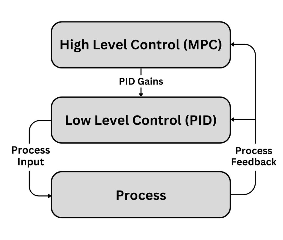
Model Predictive Control (MPC) is another advanced tuning technique. Unlike other methods that rely on heuristic rules, MPC utilizes a dynamic process model to predict future process output. This prediction is then used to optimize the future control action, minimizing the deviation from the setpoint over a future horizon. Given the complexity of the optimization problem, MPC requires significant computational resources, making it more suitable for slow processes or when high performance is required.
The relay feedback method is a frequency-domain approach to PID tuning that uses a relay (an on-off controller) to generate sustained oscillations in the system. [5] The properties of these oscillations are then used to calculate the PID parameters. One of the key advantages of this method is that it does not require a mathematical model of the process. However, it requires a process that can tolerate the induced oscillations without causing damage or safety issues.
Finally, in recent years, artificial intelligence and machine learning techniques, such as reinforcement learning and genetic algorithms, have been applied to PID tuning. These methods can adaptively tune the PID parameters to optimize performance without requiring explicit mathematical models. While these methods are promising, they require large amounts of data and computational resources, and their use in industry is still limited.
The selection of an appropriate tuning method depends on the specific characteristics of the system, the available resources, and the desired performance. Advanced methods generally require more computational resources and a deeper understanding of control types, but they can offer significant performance improvements for challenging control problems.
Application Examples of PID Control
PID Control in Industry
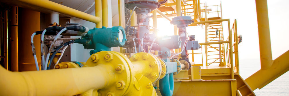
The applications of PID control are extensive in the industrial sector. Around 95% of the closed loop system of the industrial automation sector use PID controllers. A prevalent area is in the process industry, where PID controllers maintain the consistency of vital variables. FMI states that the top three applications for PID controllers are temperature control, pressure control, and flow control. Chemical industry, oil and gas industry, and power industry use PLCs to control the above parameters.
Consider a chemical reactor where a PID controller maintains a specific temperature to ensure optimal chemical reaction. The controller takes the temperature reading from a sensor within the reactor as feedback and compares it with the desired setpoint. Any deviation prompts an action, adjusting the heat input to the reactor. This is done using programmable logic controllers. In this scenario, an aggressively tuned proportional band minimizes the error but can lead to constant cycling around the setpoint. Therefore, an integral term is included to counteract bias. But a fast response could lead to instability due to the integral windup; hence a derivative component is added to dampen the response.
In manufacturing industries, PID controllers play a central role in automated systems. Take, for example, a conveyor system in an automotive assembly line. A PID controller controls the speed of the conveyor belt to ensure that the assembly process operates at a constant pace, with the belt's velocity measured and adjusted in real-time.
PID controllers are widely used in maintaining the electrical power industry to maintain power system stability. Voltage regulation in power generators is one application. The generator's output voltage is compared to a desired value, and the PID controller adjusts the field excitation current to maintain the output voltage at the desired level.
These examples are a testament to the versatility and robustness of PID control, facilitating its use in diverse and demanding industrial applications. The demand for PID controllers is projected to expand rapidly, with a robust CAGR of 16.3% to reach a valuation of US$ 1129 Million by 2032. [6]
PID Control in Robotics
PID controllers are instrumental in the field of robotics for precise and smooth operation, especially in motion control. It's ubiquitous in the field of autonomous vehicles, robotics arms, and quadcopters.
Autonomous vehicles employ PID controllers for trajectory tracking. Imagine a self-driving car trying to follow a specific path. The car measures its deviation from the desired trajectory, referred to as cross-track error. A PID controller then processes this error, generating a corrective steering command to minimize it. The proportional term responds to present errors, directing the car back to the path. The integral component counteracts a persistent bias, like a misalignment in the steering mechanism, causing the car to drift consistently to one side. The derivative part dampens the response to prevent overshoot and oscillations. With finely tuned PID parameters, the car smoothly follows the defined trajectory.
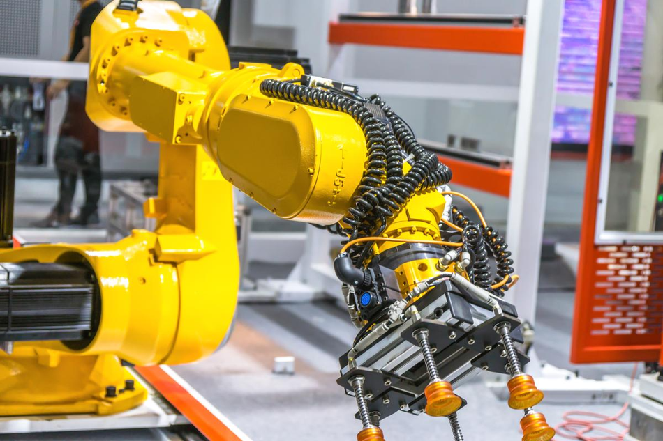
Robotic arms, especially in manufacturing, benefit from PID controllers. For a robotic arm aiming to reach a specific position, the controller compares the current position of the arm to the desired position, adjusting the motor's torque accordingly to minimize the difference. The derivative term is particularly important in this context as it accounts for the arm's rate of change in position, anticipating movements and avoiding overshoot, thus ensuring smooth and precise operations.
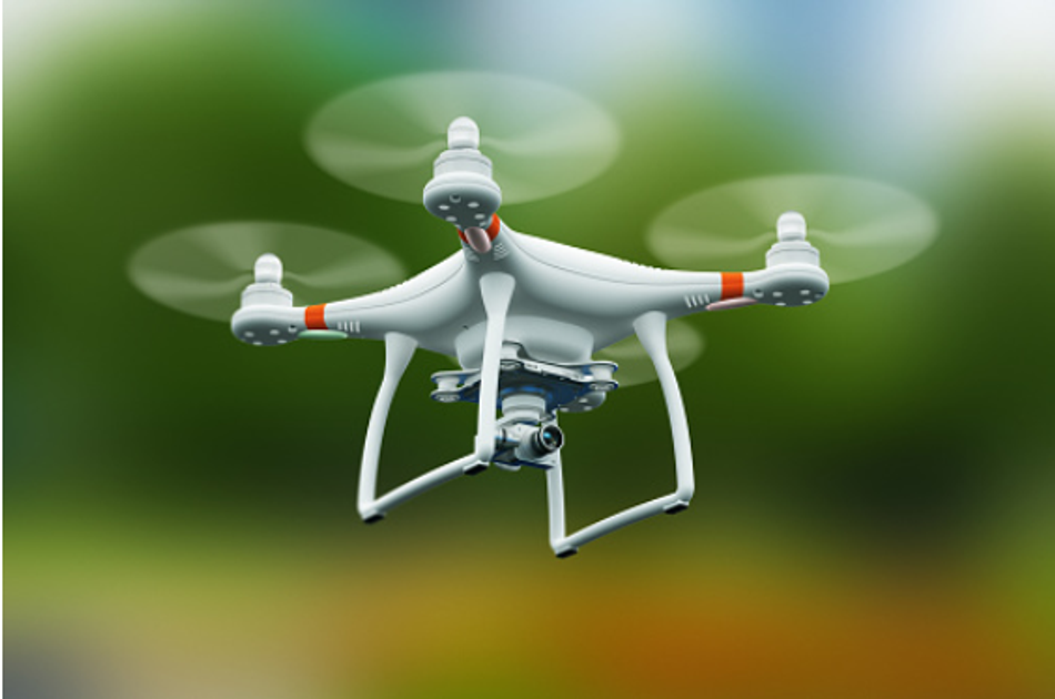
Quadcopters use PID controllers to maintain stability and execute maneuvers. A quadcopter has four rotors, and the speed of these rotors needs to be carefully controlled to achieve stable flight. By using sensors such as gyroscopes and accelerometers, the quadcopter can measure its current state (including pitch, roll, and yaw angles) and compare these with the desired states. A PID controller then calculates the difference between the current and desired states and adjusts the speed of the rotors to minimize this error. The ability of the PID controller to integrate current, past, and future errors makes it ideal for achieving stable flight and precise control in quadcopters.
The application of PID controllers in robotics showcases the versatility and effectiveness of these controllers in complex, dynamic environments where precise control and robust performance are needed.
Recommended Reading: Programmable Versus Fixed-Function Controllers: Alternatives for Complex Robotic Motion
Common Pitfalls and How to Avoid Them
While implementing PID controllers, several common pitfalls could adversely affect the performance of the control system. One such pitfall is the improper tuning of the PID parameters. If the parameters are not correctly set, the controller may not minimize the error effectively, which leads to poor system performance. This could manifest in the form of system overshoot, where the system's output goes beyond the desired setpoint, or system oscillation, where the output continuously swings above and below the setpoint. These can be mitigated by careful tuning of the PID parameters, usually starting with the proportional term, then adjusting the integral and derivative terms.
A second common pitfall is an integral wind-up, a phenomenon where the integral term accumulates an error during the period when the actuator is saturated. If unchecked, it can lead to extended periods of overshoot. Several techniques can be applied to avoid integral wind-up. These include implementing anti-windup strategies that prevent the integral term from accumulating when the actuator is at its limit.
Another pitfall is the derivative kick, which can occur when there's a sudden change in setpoint. Being sensitive to changes, the derivative term can cause a spike in output. A common approach to mitigating this is to calculate the derivative of the error instead of the setpoint, thus eliminating the impact of sudden setpoint changes on the derivative term. Labview can be used to study this derivative kick occurring in the system.
It's also worth noting that not all systems are suited for PID control. Some systems might be too complex or nonlinear for PID control to be effective, while others may not benefit from the added complexity of the integral or derivative terms. Therefore, system analysis is important before deciding to implement a PID controller.
While PID controllers are versatile and widely applicable, they aren't a panacea for all control problems. Understanding the underlying system dynamics, requirements, and limitations is essential. The adoption of PID controllers should be complemented with appropriate design methodologies, system behavior, and tuning techniques to ensure optimal performance.
Conclusion
PID control is a fundamental control technique that has found broad applicability in numerous industries, ranging from manufacturing to robotics. Its popularity stems from its simple structure, ease of implementation, and the effectiveness it offers in a wide variety of control applications. However, PID control is not without its challenges. Proper tuning of the controller's parameters is necessary to achieve optimal performance, and there are pitfalls, such as integral wind-up and derivative kick, that practitioners must be wary of. But with careful design and implementation, these issues can be mitigated, allowing the PID controller modules to perform effectively and efficiently.
FAQs
Q. What is a PID controller and how does it work?
A. A PID controller is a type of feedback controller that uses a mathematical model to regulate a process. The controller uses a control loop feedback mechanism to control the process variable and minimize the error between the desired setpoint and the actual output of a system. It does this by adjusting an input to the system based on PID.
Q. What are the components of a PID controller?
A. A PID controller consists of three components: the proportional term, the integral term, and the derivative term. The proportional term responds proportionally to the current error, the integral term accumulates past errors, and the derivative term predicts future errors based on the current rate of change. The combined action of these elements provide precise and stable control of the process.
Q. What are some common applications of PID controllers?
A. PID controllers are used in a wide variety of applications due to their effectiveness and simplicity. They are commonly used in industrial control systems to regulate temperature, pressure, flow rate, speed, and other variables. They're also widely used in robotics to control the position and velocity of robots.
Q. What are the common pitfalls in PID control, and how can they be avoided?
A. Common pitfalls in PID control include improper tuning of the PID parameters, integral wind-up, and derivative kick. These can be avoided by careful tuning of the PID parameters, implementing anti-windup strategies, and calculating the derivative of the error instead of the setpoint.
Q. Are there systems where PID control might not be suitable?
A. PID controllers are widely applicable, still they may not be suitable for all systems. Some systems might be too complex or nonlinear for PID control to be effective. In these cases, more advanced control techniques might be required.
References
1. Viechi. Work Principle of PID Control Algorithm. [Cited 2023 May 27] Available from: Link
2. Wikipedia. PID controller [Cited 2023 June 15] Available from: Link
3. George Ellis, in Control System Design Guide (Fourth Edition), Article: 6.4.1.3 The Ziegler–Nichols Method [Cited 2023 June 15] Available from: Link
4. National Instruments. Cohen-Coon Autotuning Method. [Cited 2023 June 15] Available from: Link
5. ScienceDirect. Relay feedback auto-tuning of process controllers — a tutorial review [Cited 2023 June 15] Available from: Link
6. Fortune Business Insights. PID controller market size and share | Forecast report 2029 [Cited 2023 June 15] Available from: Link