What Is Unsupervised Learning? Types, Algorithms, and Examples (2026)
Unsupervised learning is a machine learning approach that finds patterns, structure, or useful representations in unlabeled data. It groups similar observations, compresses high-dimensional features, detects outliers, discovers item relationships, and supports modern representation learning.

Last updated on 11 Aug, 2026. 15 minutes read
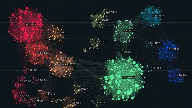
Clustering - A Common Unsupervised Learning Technique
Key Takeaways
Unsupervised learning trains on unlabeled data, so the objective is discovery rather than prediction against a known target.
The four core task types are clustering, dimensionality reduction, association rule learning, and anomaly detection.[1]
K-means, hierarchical clustering, DBSCAN, Gaussian mixture models, PCA, t-SNE, UMAP, autoencoders, Apriori, and FP-growth are among the most important practical algorithms.[1]
Evaluation is harder than in supervised learning because there is often no ground truth, so engineers combine internal metrics, visual inspection, stability checks, and downstream validation.
In 2025 and 2026, unsupervised learning is tightly connected to self-supervised learning, embeddings, and foundation model pretraining.[2]
Classical unsupervised methods remain useful because they make large embedding spaces, sensor streams, transactions, and biological datasets easier to inspect and act on.
Introduction
Unsupervised learning is used when the data exists, but the answers do not. For example, an engineering firm may have years of vibration readings from rotating equipment but only a small number of labeled failures. Likewise, a retailer may have millions of purchase baskets but no predefined customer groups. A bioinformatics team may have high-dimensional gene expression profiles but no complete taxonomy of disease subtypes. In each case, the value is not in mapping inputs to known labels. It is in discovering structure.
The uncertainty in output and lack of labeled data make unsupervised learning one of the most important branches of modern machine learning. It guides modern designers in the exploration, compression, segmentation, anomaly detection, recommendation, and feature learning.[1]
More importantly, modern unsupervised learning algorithms can be applied directly to tabular, image, text, graph, signal, or transaction data. Hence, it is applied to learned embeddings generated by deep learning models and foundation models.
What Is Unsupervised Learning?
Unsupervised learning is an umbrella of techniques where algorithms let machines learn from unlabeled data. It’s a pivotal field in data science, which lets machines identify hidden patterns in data.
Think of supervised learning, which works with labeled datasets. In a labeled dataset, each training example has an associated target, such as "defective" or "not defective," "cat" or "dog," or a numeric value such as remaining useful life.
On the contrary, in an unlabeled dataset, the model receives only the inputs. It must infer patterns from the geometry, density, similarity, co-occurrence, or reconstruction properties of the data.[3] The output depends on the task, and each algorithm has its unique mechanism for learning. For instance:
A clustering model might assign each observation to a group.[4]
A dimensionality reduction model might transform a larger number of features into fewer latent variables to reduce processing overhead and simplify processing.[5]
An anomaly detector might assign a risk score to each transaction.
An association rule model might discover that items A and B frequently appear with item C.
A representation learning model might produce embeddings that can be reused for search, recommendation, classification, or control.[6]
Unsupervised learning does not mean the model has no objective.
K-means minimizes within-cluster variation.[7]
PCA preserves as much variance as possible in fewer dimensions.[8]
Autoencoders compress and create new representations of input data, particularly for neural networks, and minimize reconstruction error.[1]
Self-supervised models solve proxy tasks such as predicting missing tokens, reconstructing masked image patches, or aligning paired text and image embeddings. It deals with complex tasks associated with training hyperparameters.[9]
Suggested Reading: Improving Dataset Creation for Machine Learning
Unsupervised vs. Supervised vs. Reinforcement Learning
Unsupervised learning is easiest to understand by comparing it with supervised learning and reinforcement learning. The three paradigms differ in the type of feedback they use.
Aspect | Supervised learning | Unsupervised learning | Reinforcement learning |
Training data | Labeled examples with inputs and known outputs | Unlabeled examples with inputs only | Interaction data from an environment |
Main goal | Learn a mapping from inputs to targets | Discover structure, groups, representations, rules, or outliers | Learn actions that maximize cumulative reward |
Feedback signal | Correct answer, label, or target value | Internal objective derived from the data | Reward or penalty after actions |
Typical output | Class label, probability, forecast, or regression value | Cluster assignment, embedding, compressed feature set, rule, or anomaly score | Policy, value function, or action strategy |
Example task | Predict whether a part will fail within 30 days | Group similar operating profiles in machine telemetry | Train a robot to optimize a pick-and-place sequence |
Evaluation | Accuracy, F1 score, ROC-AUC, mean absolute error, or similar metrics | Silhouette score, reconstruction error, likelihood, stability, visual inspection, downstream performance | Average return, regret, sample efficiency, safety constraints |
A single system can use all three machine learning mechanisms. For example, a predictive maintenance platform might use unsupervised clustering to identify equipment operating modes, supervised learning to estimate failure risk, and reinforcement learning to optimize maintenance scheduling.
In many production machine learning systems, these categories are often complementary rather than mutually exclusive.
Recommended Reading: Unsupervised Learning vs Supervised Learning
Types of Unsupervised Learning
The standard machine learning taxonomy includes four task families:
Clustering
Dimensionality Reduction
Association rule learning
Anomaly detection
This section discusses a breakdown for each type.
Clustering
Clustering is used to group data points so that items within the same group are more similar to each other than to items in other groups.[4] It is used when the natural categories are unknown or when manually defining them would be too rigid.
The best use case for clustering is when you need to segment customers, discover operating modes in sensor data, group similar documents, identify subtypes in medical or biological data, or organize large collections of embeddings.
Clustering is especially useful during exploratory analysis because it can expose structure that was not encoded in the original dataset.
The main design choice is the definition of similarity. For tabular data, this may be Euclidean distance after feature scaling. For time series, it may require dynamic time warping or learned sequence embeddings. A poor distance metric will produce poor clusters even if the algorithm is well implemented.
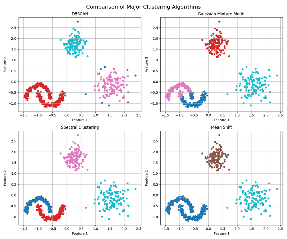
There is a wide range of clustering methods, which include K-Means, Mean-shift, spectral clustering, DBSCAN, Gaussian Mixture, and many others.[7]
Dimensionality Reduction
Dimensionality reduction transforms data from a high-dimensional space into a lower-dimensional one while preserving useful information. It reduces computational cost, removes noise, visualizes complex data, and generates compact features for downstream models.[5]
Dimensionality reduction is best applicable when the number of features is large relative to the number of samples, when features are highly correlated, or when a two-dimensional or three-dimensional visualization would help engineers inspect structure. It’s typically used in the pre-processing data stage for image analysis, genomics, sensor fusion, materials informatics, and embedding analysis.[1]
There are two broad approaches.
Linear methods, such as PCA, assume that important structure can be captured by linear combinations of original features.[8]
Nonlinear methods, such as t-distributed Stochastic Neighbor Embedding (t-SNE), UMAP, and autoencoders, can capture more complex manifolds but are more sensitive to hyperparameters and interpretation.[10,11]
Association Rule Learning
Association rule learning discovers items, events, or attributes that frequently occur together. It finds relationships between variables of a given dataset.[1] It is usually expressed as rules such as "if A and B occur, C is likely to occur."
The classic use case is market-basket analysis, but the same logic applies to spare-parts orders, alarm logs, medical codes, web sessions, and manufacturing defect combinations.
Association rule learning is best suited when the data is transactional or event-based, and the goal is to find interpretable co-occurrence patterns. The key metrics are support, confidence, and lift.
Support measures how often an itemset appears.
Confidence measures how often the rule consequent appears when the antecedent appears.
Lift measures whether the relationship is stronger than random co-occurrence.
Anomaly Detection
Anomaly detection identifies observations that deviate from normal patterns.[1] In many real systems, labeled anomalies are rare, delayed, ambiguous, or expensive to obtain. Unsupervised anomaly detection is useful because it can model normal behavior and flag unusual cases without requiring a large labeled anomaly dataset.[12]
Typically, anomaly detection is best for fraud detection, cybersecurity, quality inspection, equipment monitoring, sensor fault detection, medical screening, and network monitoring.
The output is usually not a final classification. It is a score or ranking that helps prioritize investigation. By tuning the thresholds based on risk, cost of false positives, and cost of missed anomalies, designers can better evaluate the anomalies identified by such detection algorithms.[12]
Core Unsupervised Learning Algorithms
Each algorithm makes assumptions about cluster shape, density, feature geometry, or data distribution.[7] Since there are several such algorithms, the choice of an appropriate option depends on whether these assumptions match the problem.
K-means Clustering
K-means is the standard baseline for clustering numeric data. It divides the observed values into ‘k’ clusters, repeatedly assigning each point to the nearest centroid. Each centroid is then updated to the mean of its assigned points.[1] Intuitively, it tries to place k prototypes in the data so that points are close to their assigned prototype.
K-means is fast, scalable, and easy to explain. There are several application areas for this algorithm.[4] Some of its major application areas include:
Customer segmentation
Document or image embedding grouping
Color quantization
Finding operating regimes in equipment telemetry.
Text clustering in Natural Language Processing (NLP)
Mini-batch k-means can handle large datasets by updating centroids from small random batches.
Its main limitation is its geometry. K-means works best when clusters are compact, roughly spherical, and similar in size. It also requires the engineer to choose k in advance, and it is sensitive to feature scaling and outliers. In practice, teams often run k-means multiple times with different random initializations and compare inertia, silhouette score, and business interpretability.
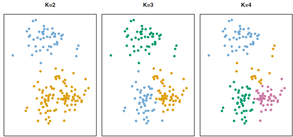
A good K-Means clustering algorithm creates clusters that have the minimum within-cluster variation. For this purpose, there are several techniques to measure the distance between the observations in each cluster, such as:
- Euclidean Distance - Computes the square root of the square of the distances between coordinate pairs of objects.
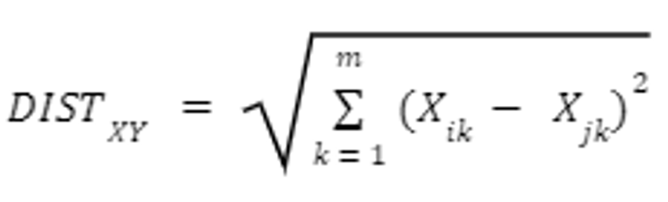
- Manhattan Distance - Computes the absolute distance between object pairs
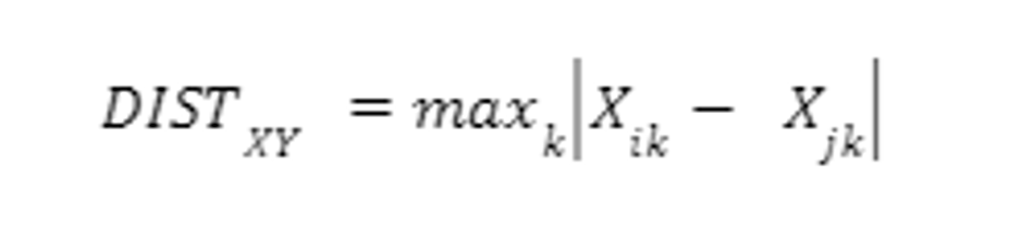
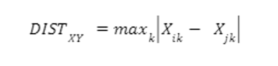
- Chebyshev Distance - Computes the absolute magnitude of the difference between object pairs.
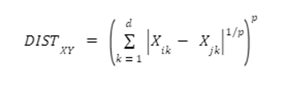
- Minkowski Distance - Calculates generalized metric distance
Hierarchical Clustering
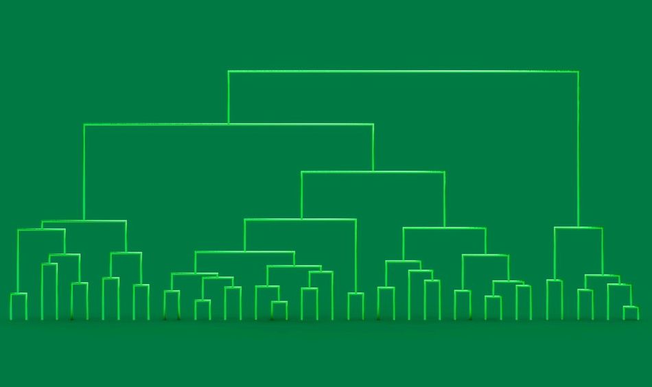
Hierarchical clustering builds a nested tree of clusters, where each point begins as its own cluster. The algorithm repeatedly merges the closest clusters.[7] Hierarchical clustering can be either agglomerative (bottom-up) or divisive (top-down).
Agglomerative Clustering: each data point starts as its cluster, and the algorithm iteratively merges the closest pairs of clusters until only one cluster remains.
Divisive Hierarchical Clustering: starts with a single cluster containing all data points and recursively splits the clusters until each data point forms its cluster.
The result is a dendrogram that shows how clusters combine at different similarity thresholds.
This is useful when the hierarchy itself matters. Engineers may use it to build taxonomies of failure modes, group materials by measured properties, organize biological samples, or inspect small to medium-sized datasets where interpretability matters more than raw speed.
The key design choice is linkage, which includes:
Single linkage to find elongated structures but may chain through noise.
Complete linkage for compact clusters.
Average and Ward linkage are common practical choices.
Hierarchical clustering can be computationally expensive on large datasets, so it is often applied after sampling, dimensionality reduction, or embedding generation.
DBSCAN
DBSCAN, short for density-based spatial clustering of applications with noise, finds dense regions separated by sparse regions.[13]
It uses two main parameters:
Epsilon: defines the neighborhood radius
Minimum Samples: defines the required number of neighbors for a point to be considered part of a dense region.
It works on a simple intuition that the points in crowded neighborhoods become cluster cores. The nearby points join those clusters, and isolated points are marked as noise. Unlike k-means, DBSCAN does not require the number of clusters in advance and can find non-spherical clusters.
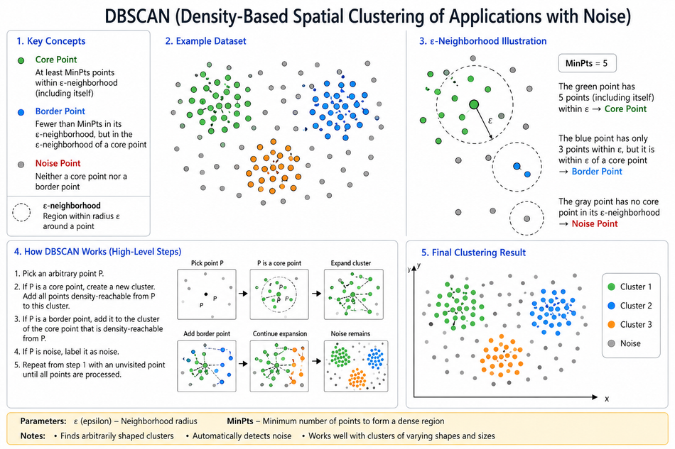
DBSCAN is useful for spatial data, geolocation patterns, sensor events, and anomaly detection where noise points are meaningful.[13]
But it struggles when clusters have very different densities or when distance becomes less meaningful in high-dimensional spaces. Also, it is largely dependent on parameter tuning, because a small change in epsilon can change the clustering substantially.
Gaussian Mixture Models
Gaussian mixture models, or GMMs, treat the data as a combination of multiple Gaussian distributions. Instead of assigning each point to exactly one cluster, a GMM gives each point a probability of belonging to each component.[14]
GMMs are useful when clusters overlap, have elliptical shapes, or need probabilistic interpretation. They are often fitted using expectation-maximization, an iterative procedure that alternates between estimating component memberships and updating component parameters.
GMMs can also support anomaly detection by flagging points with low probability under the learned distribution.[14] Also, they are more assumption-driven and allow the data to be modeled as a mixture of Gaussian components.
Principal Component Analysis
Principal component analysis, or PCA, is the canonical linear dimensionality reduction method.[15] It finds new orthogonal axes, called principal components, that capture the maximum variance in the data.[1] By keeping only the first several components, PCA can reduce dimensionality while preserving much of the dataset's variation.
PCA is useful for compression, denoising, visualization, exploratory analysis, and preprocessing before clustering or supervised modeling.[15] It is particularly effective for correlated features such as sensor channels, spectral measurements, and those obtained from feature engineering.
PCA is not a universal structure detector. It captures variance, not necessarily task relevance. It is linear, sensitive to scaling, and can be distorted by outliers.
t-SNE and UMAP
t-SNE and UMAP are nonlinear dimensionality reduction methods widely used for visualizing high-dimensional data in two or three dimensions.[10] They are especially common for image embeddings, text embeddings, single-cell biology data, and other datasets where local neighborhoods matter.
t-SNE focuses on preserving local neighbor relationships. It can produce clear visual separation between groups, which makes it useful for exploratory plots.[16] A critical aspect of the t-SNE algorithm is proportionality. Two groups that appear far apart are not necessarily proportionally far apart in the original space. Therefore, global distances and cluster sizes in a t-SNE plot can be misleading.
UMAP also builds a neighborhood graph and optimizes a low-dimensional layout. It is often faster than t-SNE on large datasets and can preserve more global structure in many practical settings. UMAP can also be used as a general feature transformation, but its output still needs validation.[11]
Hence, a practical rule is to treat t-SNE and UMAP plots as maps for exploration, not as proof. They are excellent for generating hypotheses about structure, but the final interpretation should be checked with metrics, domain knowledge, and downstream tests.
Autoencoders
Autoencoders are unsupervised or self-supervised neural networks trained to reconstruct their input. The encoder compresses the input into a latent representation, and the decoder reconstructs the original data from that representation.[1] If the latent representation is constrained, the model must learn the most important structure needed for reconstruction.
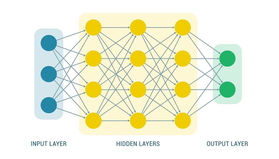
Autoencoders are useful for nonlinear dimensionality reduction, denoising, feature learning, anomaly detection, and pretraining. In anomaly detection, the idea is that a model trained on normal data will reconstruct normal inputs well but reconstruct unusual inputs poorly, producing a high reconstruction error.
Apriori and FP-growth
Apriori and FP-growth are the classic algorithms for frequent itemset mining and association rule learning. Apriori uses the principle that if an itemset is frequent, all of its subsets must also be frequent.[1] It generates candidate itemsets level by level and prunes candidates that cannot meet the minimum support threshold.
FP-growth takes a different approach. It compresses the transaction database into a frequent-pattern tree and mines frequent itemsets without generating large candidate sets.[1]
These algorithms are useful for interpretability. For example, a maintenance team might discover that certain alarms, spare parts, and environmental conditions co-occur before a failure. A retailer might discover product bundles. Likewise, a cybersecurity team might find recurring combinations of events in intrusion traces.
Unsupervised Learning Applications
Customer Segmentation
Customer and market segmentation is one of the clearest business uses of clustering. Unsupervised learning allows businesses to autonomously segment customer groups. These groups or segments may be based on age, region, or account size. It can group customers by behavior, purchase history, product usage, support interactions, or engagement patterns.[1]
Especially for engineering firms, unsupervised learning can reveal groups like high-utilization customers, maintenance-sensitive customers, customers likely to need spare parts, or users adopting a product in unexpected ways.
Anomaly and Fraud Detection
Fraud and anomaly detection often suffer from label scarcity. True fraud labels may arrive late after investigation. Equipment failures may be rare.[1] Cybersecurity attacks may evolve faster than labeled datasets can be collected.
A practical system typically combines unsupervised scoring with human review, rule-based safeguards, and supervised models once enough labels become available.
Bioinformatics and Scientific Discovery
Bioinformatics is a natural fit for unsupervised learning because many datasets are high-dimensional and only partially labeled. Gene expression, single-cell RNA sequencing, protein measurements, and imaging assays can contain thousands of features per sample.
Clustering can identify cell types or disease subgroups. Dimensionality reduction can make high-dimensional biological structure visible. For instance, enhanced image segmentation models can help improve the efficiency of ML algorithms in early detection and pre-processing of data, feature extraction, and segmentation.[17]
Recommended Reading: A new computational model can predict antibody structures more accurately
Recommendation and Discovery
Recommendation systems often use unsupervised structure even when they also use supervised objectives. Clustering can group similar users or items. Matrix factorization and embedding methods can place users and items in the same latent space. Association rules can expose products or events that frequently occur together.
For example, an engineering parts marketplace might use association rules to identify components often purchased together, embeddings to retrieve similar parts, and clustering to organize a large catalog into functional families. The strongest recommendation systems usually combine multiple signals rather than relying on one algorithm.
Suggested Reading: AI and machine learning goes mainstream
Challenges with Unsupervised Learning
No Ground Truth
The central evaluation problem is that there may be no correct answer. If an algorithm returns seven clusters, it is not obvious whether seven is better than five or whether the clusters correspond to anything meaningful.[18]
Engineers use several validation strategies. Internal metrics such as silhouette score, Davies-Bouldin index, and Calinski-Harabasz score measure cluster compactness and separation. Reconstruction error can evaluate autoencoders or PCA.
Dimensionality Issues
As dimensionality increases, distances often become less informative. Points may appear similarly far apart, neighborhoods become sparse, and density estimates become unreliable. This weakens clustering, nearest-neighbor search, and anomaly detection.
The practical response is to reduce dimensionality, learn better representations, remove irrelevant features, standardize units, and use domain knowledge to design meaningful features.
Interpretability
Unsupervised outputs can be difficult to explain. A supervised classifier predicts a known label. A cluster, latent variable, or embedding dimension may not have a direct physical meaning. This can create problems in regulated, safety-critical, or customer-facing systems.[18]
Interpretability improves when teams profile clusters using original features, inspect representative examples, compare distributions across groups, and name clusters only after validation.
Self-Supervised Learning, Embeddings, and Foundation Models in Modern Context
The meaning of unsupervised machine learning has expanded. Classical articles often focused on clustering and dimensionality reduction. Those methods are still important, but the center of gravity has shifted toward representation learning.[2]
Self-supervised learning is the most important bridge. In self-supervised learning, labels are generated automatically from the data.
A language model predicts the next token or masked tokens.
A vision model reconstructs masked patches or learns that two augmented views come from the same image.
A multimodal model learns to align images with captions.
The training data is not labeled in the traditional supervised sense, but the model still receives a learning signal created from the structure of the data.[1] This is why modern foundation models are closely related to unsupervised learning. They are pretrained on broad datasets at scale, often with self-supervised objectives, and then adapted to downstream tasks through prompting, fine-tuning, retrieval, adapters, or supervised instruction tuning.
The 2025-2026 context is not that classical unsupervised learning has been replaced. It is that classical methods now operate at a higher level of abstraction. They help engineers inspect, compress, cluster, and monitor learned representation spaces.
Recommended Reading: Meta AI Introduces Data2vec Open-Source Framework for Self-Supervised Learning in NLP, Speech and Vision Processing
Conclusion
Unsupervised learning discovers structure in unlabeled data. Its main task types are clustering, dimensionality reduction, association rule learning, and anomaly detection. Its core algorithms range from simple and interpretable methods such as k-means, PCA, hierarchical clustering, and the Apriori algorithm to more flexible methods such as DBSCAN, Gaussian mixture models, UMAP, and autoencoders.
The practical value is not just automation. It is visibility. Unsupervised learning helps engineers understand complex datasets, compress high-dimensional signals, identify unusual behavior, organize embeddings, discover co-occurrence patterns, and create features for downstream models.
In 2026, unsupervised learning should be understood in both its classical and modern forms. Classical methods remain essential for segmentation, visualization, and anomaly detection. Self-supervised pretraining and representation learning now underpin many foundation models.
Frequently Asked Questions
1. What is unsupervised learning?
Unsupervised learning is a machine learning approach that finds patterns in unlabeled data. It does not train on examples with known answers. Instead, it discovers clusters, lower-dimensional representations, association rules, anomaly scores, or embeddings based on the structure of the input data.
2. What is the difference between unsupervised vs supervised learning?
Supervised learning uses labeled data, where each training example has a known target. The goal is to predict that target for new examples. Unsupervised learning uses unlabeled data and tries to discover structure, such as groups, patterns, or compressed representations. In practice, unsupervised learning is often used before supervised learning to explore data or create features.
3. What are examples of unsupervised learning?
Common examples include customer segmentation with k-means, anomaly detection in sensor data, PCA for reducing high-dimensional measurements, t-SNE or UMAP for visualizing embeddings, association rule mining for product bundles, autoencoders for feature learning, and clustering gene expression profiles in bioinformatics.
4. Is clustering supervised or unsupervised?
Clustering is generally unsupervised. It groups unlabeled examples based on similarity rather than learning from predefined class labels. If labels are available and the model learns to assign new examples to those known labels, the task is classification, not clustering.
References
IBM, “What is unsupervised learning?” [Online]. Available: https://www.ibm.com/think/topics/unsupervised-learning
Stanford HAI, “The 2025 AI Index Report.” [Online]. Available: https://hai.stanford.edu/ai-index/2025-ai-index-report
C. M. Bishop, Pattern Recognition and Machine Learning. Springer. [Online]. Available: https://link.springer.com/book/9780387310732
Google for Developers, “What is clustering?” [Online]. Available: https://developers.google.com/machine-learning/clustering/overview
scikit-learn, “Unsupervised dimensionality reduction.” [Online]. Available: https://scikit-learn.org/stable/modules/unsupervised_reduction.html
Y. Bengio, A. Courville, and P. Vincent, “Representation Learning: A Review and New Perspectives,” IEEE Transactions on Pattern Analysis and Machine Intelligence, vol. 35, no. 8, pp. 1798–1828, 2013. [Online]. Available: https://ieeexplore.ieee.org/document/6472238
scikit-learn, “Clustering user guide.” [Online]. Available: https://scikit-learn.org/stable/modules/clustering.html
scikit-learn, “PCA API reference.” [Online]. Available: https://scikit-learn.org/stable/modules/generated/sklearn.decomposition.PCA.html
R. Balestriero et al., “A Cookbook of Self-Supervised Learning,” arXiv:2304.12210. [Online]. Available: https://arxiv.org/abs/2304.12210
scikit-learn, “t-SNE API reference.” [Online]. Available: https://scikit-learn.org/stable/modules/generated/sklearn.manifold.TSNE.html
L. McInnes, J. Healy, and J. Melville, “UMAP: Uniform Manifold Approximation and Projection for Dimension Reduction,” arXiv:1802.03426. [Online]. Available: https://arxiv.org/abs/1802.03426
scikit-learn, “Novelty and outlier detection user guide.” [Online]. Available: https://scikit-learn.org/stable/modules/outlier_detection.html
M. Ester, H.-P. Kriegel, J. Sander, and X. Xu, “A Density-Based Algorithm for Discovering Clusters in Large Spatial Databases with Noise,” in Proc. 2nd Int. Conf. Knowledge Discovery and Data Mining (KDD), 1996. [Online]. Available: https://cdn.aaai.org/KDD/1996/KDD96-037.pdf
scikit-learn, “Gaussian mixture models user guide.” [Online]. Available: https://scikit-learn.org/stable/modules/mixture.html
I. T. Jolliffe and J. Cadima, “Principal component analysis: a review and recent developments,” Philosophical Transactions of the Royal Society A, vol. 374, no. 2065, 20150202, 2016. [Online]. Available: https://royalsocietypublishing.org/doi/10.1098/rsta.2015.0202
L. van der Maaten and G. Hinton, “Visualizing Data using t-SNE,” Journal of Machine Learning Research, vol. 9, pp. 2579–2605, 2008. [Online]. Available: https://jmlr.csail.mit.edu/papers/v9/vandermaaten08a.html
IEEE Xplore, article available at: https://ieeexplore.ieee.org/document/10169504
IBM, “What is ground truth?” [Online]. Available: https://www.ibm.com/think/topics/ground-truth
in this article
1. Key Takeaways2. Introduction3. What Is Unsupervised Learning?Unsupervised vs. Supervised vs. Reinforcement Learning5. Types of Unsupervised Learning6. Core Unsupervised Learning Algorithms7. Unsupervised Learning Applications8. Challenges with Unsupervised Learning9. Self-Supervised Learning, Embeddings, and Foundation Models in Modern Context10. Conclusion11. Frequently Asked Questions12. References