Unsupervised vs Supervised Learning: A Comprehensive Comparison

Introduction

In artificial intelligence and machine learning, two primary approaches stand out: unsupervised learning vs supervised learning. Both methods have distinct characteristics and applications, making it crucial for practitioners to understand their differences and choose the most suitable approach for solving problems. 

While unsupervised learning involves discovering patterns and structures within data without prior knowledge of the desired output, supervised learning relies on labeled data to train models to make predictions or classifications. This guide on unsupervised vs supervised learning will elaborate on the nuances of these two techniques, allowing machine learning practitioners to effectively leverage their strengths and address the challenges posed by various real-world problems. 

What is Supervised Learning?

Supervised learning is a type of machine learning where an algorithm learns from a dataset containing input-output pairs, also known as labeled data. It aims to create a model that can make accurate predictions or classifications based on new, unseen input data. The learning process involves using the input dataset to train an algorithm model and adjusting its weights until they fit the training model perfectly. 

Eventually, it narrows the gap between parameters to minimize the difference between the predicted outputs and the actual outputs in the dataset.

Example of Supervised Learning

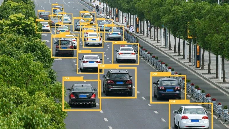
A typical example of supervised machine learning is the identification of images. Imagine there are two animals, a dog, and a cat. To help the machine understand the differences, it must first learn what each animal looks like. 

So, the machine is trained by providing several pictures of dogs and cats, and it starts learning the patterns and features from each image. Each image is labeled 'Dog' or 'Cat' so the machine can understand and update its parameters for each class. 

With the help of more images, the machine can learn better by extracting the features closely and identifying the animal more accurately. 

That's why selecting features is a crucial aspect of supervised learning. Likewise, feature selection and feature engineering play a crucial role in the success of a supervised learning model because they significantly impact the model's ability to learn and make accurate predictions.

With time, supervised learning improves the accuracy and efficiency of a machine learning model as it continues to learn from updated datasets. It's one of the reasons that supervised learning is a viable option in assembly lines where robotic imaging and automation are intended. Likewise, it has applications in fraud detection, autonomous vehicles, and automated systems.

Recommended reading: Supervised Learning is Critical to the Future of Automation

The Role of Datasets in Supervised Learning

In supervised learning, every dataset is divided into two parts: 

• Training set - it is used to train the model

• Testing Dataset - used to test the model. 

In addition to the performance metrics, the accuracy of a supervised learning model heavily depends on the size and quality of a training set. 

For instance, the size of a training dataset determines how accurately it can predict the output in various applications. Here, it's critical to understand the application of the algorithm, and the size of training sets can vary accordingly. 

Size of a Dataset

For example, the Iris Flower dataset contains 150 samples of three Iris flower species. It's primarily used for testing classification algorithms, feature selection, dimensionality reduction, and data visualization. 

On the other hand, the Google Translate dataset contains trillions of examples, given that it needs such humongous data to predict translations for more than 130 global languages accurately. 

Dataset Quality

The dataset quality is the other essential feature. Regardless of the dataset size, the quality of data determines the precision of a supervised learning model. If the data quality isn't excellent, it can never produce accurate results, no matter how much data it has been trained on. The quality of a dataset has three essential aspects:

• Reliability 

• Skew Minimization

• Feature Representation

The training set is used to train the model, while the testing set is used to evaluate the model's performance. 

Performance Analysis of Supervised Learning Models

The performance of a supervised learning model is typically measured using metrics such as 

• Accuracy 

• Precision 

• Recall 

• F1 score

• Log Loss

These metrics help determine how well the model generalizes to new data and can be used to fine-tune the model's parameters for optimal performance. 

Moreover, since supervised learning is based on predicting true and false results, it introduces the concept of a Confusion Matrix. Understanding the confusion matrix is critical in analyzing the performance metrics of a supervised learning model. 

What is a Confusion Matrix?

The confusion matrix is an NxN matrix that indicates the label of a specific output from a machine learning model. So, there is an actual label and a predicted label. 

So, imagine a 2x2 confusion matrix having the actual label on the y-axis and the predicted label on the x-axis. Each label could have either a true or a false output.

Every time the model makes a prediction, it will show one of the results from TP, TN, FP, and FN. To better understand these outputs, let's assume a term: "If the detected image is a boy or a girl."

Positive - Detected Image is a boy

Negative - Detected Image is a girl

True Positive (TP) - Predicted image is a boy, and the actual image is also a boy. It means that the model correctly predicted the results. It represents that the predicted and actual labels are both positive.

True Negative (TN) - The predicted image is a girl, and the actual image is a girl. Once again, the model correctly predicted the results. It shows that the predicted and actual labels are both negative.

False Positive (FP) - The predicted image is a boy, but the actual image is a girl. In this case, the model wrongly predicts the result. 

False Negative (FN) - The predicted image is a girl, but the actual image is a boy. Once again, the model predicts the wrong result.

Types of Supervised Learning

Classification

Classification is a supervised learning task that assigns input data to one of several predefined categories or classes. So, when a classification model learns a new observation, it classifies the input into any of the preexisting categories provided in the training dataset. 

That's why classification problems produce a definite output. Meaning it can take on a limited number of discrete values. 

Examples of classification include:

• Spam detection - where emails are classified as spam or not spam

• Image recognition - where images are classified, such as animals, vehicles, or people.

Various algorithms are used for classification tasks, including logistic regression, support vector machines, decision trees, and neural networks. 

Performance Evaluation of a Classification Model

Typically, classification models are evaluated with performance metrics like precision, accuracy, recall, and F1 score because these metrics evaluate the ability of the model to predict and categorize new data points. 

Additionally, it is crucial to consider the balance of classes in the dataset, as imbalanced datasets can lead to biased models that favour the majority class. Techniques such as oversampling, undersampling, and synthetic data generation can be employed to address class imbalance and improve model performance.

Fig 1: Pattern Classification  

Regression

Regression is a supervised learning task that predicts continuous numerical values based on input data. 

Regression models work on continuous values, i.e., the output, also known as the target variable, is a continuous numerical value. This is the critical differentiator between Regression and classification models. 

Regression aims to create a model that can accurately predict the target variable for new, unseen input data.

Various regression models include:

• Linear Regression - a statistical model that establishes a linear relationship between a dependent variable and one or more independent variables, aiming to predict or explain the dependent variable based on the values of the independent variables.

• Polynomial Regression - an extension of linear regression that models the relationship between a dependent variable and independent variables by fitting a polynomial equation to the observed data, accommodating non-linear patterns and allowing for more flexible predictions.

• Ridge and Lasso Regression - regularization techniques to prevent overfitting by introducing additional penalty terms. Ridge regression uses L2 regularization, and Lasso regression uses L1 to constrain the model's coefficients during training.

Common Supervised Learning Algorithms

Linear Regression

Linear regression is used to predict a continuous target variable based on one or more input features. The algorithm assumes a linear relationship between the input features and the target variable, which can be represented by a straight line in the case of a single input feature or a hyperplane in the case of multiple input features.

The linear regression model can be expressed mathematically as follows:

y = β0 + β1x1 + β2x2 + ... + βnxn + ε

Where y is the target variable, x1, x2, ..., xn are the input features, β0 is the intercept, β1, β2, ..., βn are the coefficients, and ε is the error term.

The Goal of Linear Regression

Linear regression aims to find the optimal values for the coefficients that minimize the sum of the squared differences between the predicted values and the actual values in the dataset. This optimization problem is typically solved using gradient descent or the standard equation.

The algorithm is sensitive to outliers and the assumption of a linear relationship between the input features and the target variable. That's why linear regression models don't work efficiently in complex machine learning applications. 

Logistic Regression

Logistic regression is used for binary classification tasks. The algorithm predicts one of two possible outcomes based on input features. It only predicts the probability of an input belonging to a specific class. 

The algorithm is an extension of linear regression, using the logistic function (also known as the sigmoid function) to transform the linear regression output into a probability value between 0 and 1.

The logistic function is defined as:

σ(z) = 1 / (1 + exp(-z))

Where z is the linear combination of input features and their corresponding coefficients, similar to the linear regression equation.

The logistic regression model can be expressed mathematically as follows:

P(y=1|x) = σ(β0 + β1x1 + β2x2 + ... + βnxn)

P(y=1|x) is the probability that the target variable y equals 1 given the input features x1, x2, ..., xn, and β0, β1, ..., βn are the coefficients.

The Goal of Logistic Regression

Logistic regression finds the optimal values for the coefficients that maximize the likelihood of the observed data. This optimization problem is typically solved using gradient descent or Newton-Raphson method.

Logistic regression is sensitive to outliers and assumes a linear relationship between target variables and input features. Moreover, it inflates standard error and variance when working with multi-collinear points and data. It’s helpful because of its simplicity, interpretability, and ability to handle linear and non-linear relationships between input features and the target variable. 

Support Vector Machines

Support Vector Machines (SVM) is a robust algorithm for classification and regression tasks. The primary goal of SVM is to find the optimal decision boundary, known as the maximum-margin hyperplane, that separates the different classes or predicts the target variable with the highest possible margin.

The data points closest to the decision boundary, called support vectors, determine the maximum-margin hyperplane. The support vectors define the margin and influence the position of the decision boundary. 

The margin is the distance between the decision boundary and the support vectors, and SVM aims to maximize this margin to improve the model's generalization ability.

• SVM can handle linear and non-linear relationships between input features and the target variable. 

• For non-linear problems, SVM uses the kernel trick, which maps the input data into a higher-dimensional space where a linear decision boundary can be found. 

• It commonly uses functions like linear kernel, polynomial kernel, radial basis function (RBF) kernel, and sigmoid kernel.

• SVM can handle high-dimensional data without overfitting and flexibly models linear and non-linear relationships. 

Limitations of Support Vector Machines 

SVM can be computationally expensive, especially for large datasets, and its performance is quite sensitive to the choice of kernel function and hyperparameters, such as the regularization parameter C and the kernel-specific parameters.

Typically, SVM is used for image classification, text categorization, and bioinformatics because it can handle high-dimensional data and complex relationships. 

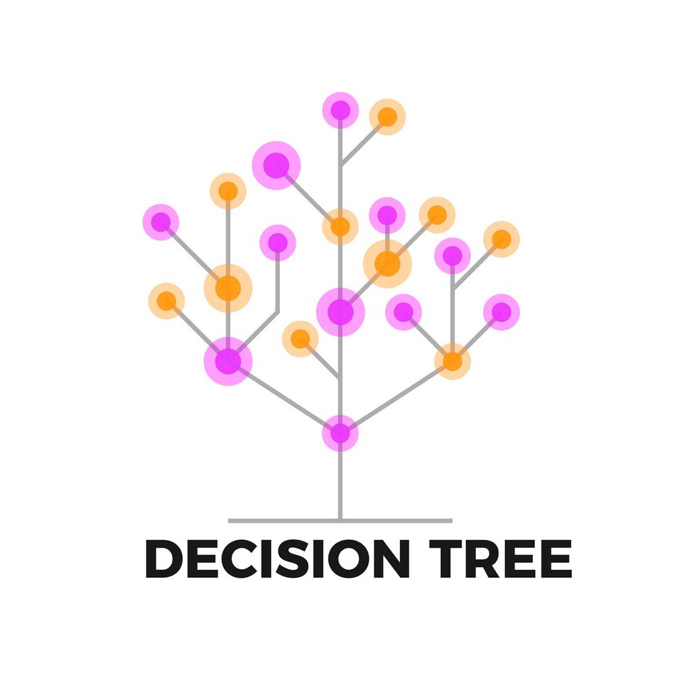
Decision Trees

Decision trees are also used for both classification and regression applications. These models  continually split the input data into subsets based on the values of the input features, creating a tree-like structure with internal nodes representing decision rules and leaf nodes representing the predicted class or value.

Eventually, it creates 

The decision rules in a decision tree are determined by selecting the input feature and the split point that results in the highest information gain or the lowest impurity, depending on the chosen criterion. 

Common criteria for splitting include Gini impurity, entropy, and mean squared error (for regression tasks). The process of splitting continues until a stopping criterion is met, such as a maximum tree depth, a minimum number of samples per leaf, or a minimum information gain.

Decision trees are highly interpretable, as humans can easily visualize and understand the decision rules. The algorithm can handle numerical and categorical input features and missing data, making them suitable for a wide range of applications. 

Limitations of Decision Trees

Decision trees are prone to overfitting, especially when the tree is deep, or the dataset is small. To avoid overfitting, there are several techniques, such as 

• Pruning 

• Limiting tree depth

• Ensemble methods like random forests and gradient boosting 

Fig 2. Decision Tree Algorithm

What is Unsupervised Learning?

Unsupervised learning involves learning from a dataset without prior knowledge of the known or desired outputs. Unlike supervised learning, there is no labeled data here.

Unsupervised learning is used to discover patterns, structures, or relationships within the data that can provide valuable insights or facilitate further analysis. 

Unlike supervised learning, focuses solely on the input data and the learning algorithm./

Components of Unsupervised Learning

The main components of unsupervised learning are the input data. It includes observations or instances and the learning algorithm responsible for extracting meaningful information from the data. 

Primarily, unsupervised learning has two significant branches i.e.

• Clustering

• Dimensionality Reduction

The techniques is primarily used for 

• Anomaly detection (to identify outlying data points)

• Feature extraction

• Generative modeling

• Natural language processing

• Data visualization and preprocessing. 

Hence, it finds vast applications in the field of computer vision, data mining, and natural language processing. With the help of unsupervised learning, researchers can better understand insights about their datasets, enabling them to design more robust and practical models for quicker learning. 

Further reading: How CAMS, the Cameras for Allsky Meteor Surveillance Project, detects long-period comets through machine learning

Types of Unsupervised Learning

Clustering

Clustering is an unsupervised learning task that aims to group similar data points based on their features without prior knowledge of the underlying structure or labels. 

Clustering models identify natural patterns and group them into clusters. For instance, clustering can be used for segmentation to analyze demographics, consumer behavior, purchasing history, and browsing behavior for a company. 

It provides insights into the relationships between data points and their features, enabling developers and researchers to devise better learning strategies.

Some of the most widely used clustering algorithms include 

• K-means Clustering - partitions a dataset into 'k' distinct clusters by iteratively assigning data points to the nearest centroid and updating the centroids based on the mean of the assigned points.

• Hierarchical Clustering - a family of clustering algorithms that build a tree-like structure of nested clusters, either through a bottom-up (agglomerative) or top-down (divisive) approach. 

• DBSCAN Clustering - groups dense regions of data points together while identifying outliers by considering the density of points in their local neighborhoods.

Dimensionality Reduction

Dimensionality reduction aims to reduce the number of features or dimensions in a dataset while preserving its essential structure or relationships. Typically, high-dimensional data takes more computational power and can be hard to analyze or visualize. 

Eventually, such data undergoes overfitting, which leads to increased computational complexity and decreased model performance. 

The idea behind dimensionality reduction techniques is to transform the data into a lower-dimensional representation that retains the most relevant information.

There are various dimensionality reduction algorithms, each with its approach to selecting or transforming features to create a lower-dimensional representation. 

While there are many dimensionality reduction techniques, the most commonly used reduction algorithms include:

• Principal Component Analysis (PCA) - finds orthogonal directions, known as principal components, that capture the maximum variance in the data.

• t-Distributed Stochastic Neighbor Embedding (t-SNE) - maps high-dimensional data into a lower-dimensional space while emphasizing the local structure and preserving clusters of similar data points.

• Linear Discriminant Analysis - finds a linear combination of features that maximizes class separability to project data onto a lower-dimensional space while preserving class discrimination.

• Independent Component Analysis (ICA) - finds statistically independent components by separating a multi-dimensional signal into its constituent components.

• Autoencoders - neural network models where the network is trained to reconstruct the input data, forcing the hidden layers to capture essential features and reduce dimensionality.

• Non-negative Matrix Factorization (NMF) - factorizes a non-negative matrix into a product of lower-rank matrices, aiming to find a parts-based representation of the data.

Common Unsupervised Learning Algorithms

K-means Clustering

K-means clustering is a widely used partition-based clustering algorithm that aims to divide the data into K distinct clusters based on their mean feature values. The algorithm works iteratively, assigning each data point to the nearest cluster centroid and updating the centroids until convergence. 

K-means clustering aims to minimize the sum of squared distances between data points and their corresponding cluster centroids.

The K-means clustering algorithm consists of the following steps:

1. Initialize K cluster centroids randomly by selecting K data points from the dataset.

2. Assign each data point to the nearest centroid.

3. Update the centroids by calculating the mean of all data points assigned to each centroid.

4. Repeat steps 2 and 3 until the centroids' positions no longer change significantly or a predefined number of iterations have been reached.

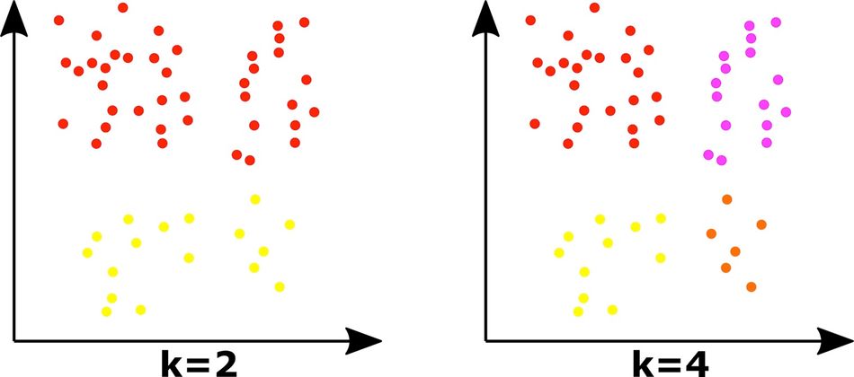
The choice of K, the number of clusters, is a critical parameter in K-means clustering. An inappropriate choice of K can lead to poor clustering results. For instance, adding more centroids tends to overfit, creating more clusters with fewer data points. It makes it harder to understand the data groups. 

Therefore, techniques like the Elbow method, silhouette analysis, and gap statistic can be used to determine the optimal value of K.

Fig 3. K-means clustering representing different values of 'k'

Limitations of K-Means Clustering

Even though K-means clustering is simplistic, scalable, and can handle larger datasets, it has a few limitations, which include:

• It's sensitive to the initial placement of centroids

• The algorithm assumes spherical clusters

• The appropriate choice of 'K' is critical

As an alternative, algorithms like K-means++ provide an improved model to overcome centroid initialization and convergence problems. 

DBSCAN 

DBSCAN (Density-Based Spatial Clustering of Applications with Noise) is a density-based clustering algorithm that groups data points based on their density in the feature space. DBSCAN defines clusters as dense regions of data points separated by areas of lower point density. 

DBSCAN clusters are much different from hierarchical and K-means cluster as they can identify arbitrary-shaped clusters. That's why they are more robust against noisy data as well. It's a competitive advantage as K-means and hierarchical clusters work efficiently only on spherical clusters.

Limitation of the DBSCAN Algorithm

While DBSCAN is quite robust to noise, it's sensitive to the choice of the distance metric and the density parameter values. Therefore, it can significantly impact the resulting clusters and make it challenging to find the optimal parameters for different types of datasets.

Hierarchical Clustering

Hierarchical clustering is a family of clustering algorithms that build a tree-like structure of nested clusters, either through a bottom-up (agglomerative) or top-down (divisive) approach. 

The output of a hierarchical clustering algorithm is a tree structure called a dendrogram. It visualizes relationships between the data points and the appropriate number of clusters. 

Agglomerative Hierarchical Clustering 

It is a bottom-up approach that starts with each data point as its cluster and iteratively merges the closest clusters until a single cluster remains. The closeness between clusters can be determined using various linkage criteria, such as single linkage (minimum distance between clusters), complete linkage (maximum distance between clusters), average linkage (average distance between clusters), and Ward's method (minimum increase in total within-cluster variance).

The agglomerative hierarchical clustering algorithm consists of the following steps:

1. Initialize each data point as its cluster.

2. Compute the distance matrix between all pairs of clusters using the chosen linkage criterion.

3. Merge the two clusters with the smallest distance.

4. Update the distance matrix to reflect the new cluster.

5. Repeat steps 2-4 until a single cluster remains.

Agglomerative hierarchical clustering produces hierarchical clusters, which can lead to the development of hierarchical structures and lets you explore various levels of granularity.

Divisive Hierarchical Clustering 

It is a top-down approach that starts with a single cluster containing all data points and recursively splits the clusters until each data point forms its cluster. 

The splitting process can be based on various criteria, such as the largest within-cluster variance or the highest dissimilarity between data points.

Limitations of Hierarchical Clustering

Hierarchical clustering has several advantages, such as its ability to generate hierarchical visual representations of the data and its flexibility in picking the appropriate number of clusters.

However, hierarchical clustering has a couple of major limitations too:

• It's quite sensitive to the choice of a linkage criterion and distance metric.

• It increases computational complexity with larger data sets.

Principal Component Analysis (PCA)

Principal Component Analysis (PCA) is a widely used linear dimensionality reduction technique that aims to transform a high-dimensional dataset into a lower-dimensional representation while preserving the maximum amount of variance in the data. PCA is particularly useful for reducing the complexity of the data, improving computational efficiency, and mitigating the effects of the curse of dimensionality.

The idea behind PCA is to identify the principal components, which are linear combinations of the original features that capture the most variance in the data. 

• The first principal component accounts for the highest variance

• The second principal component accounts for the second-highest variance orthogonal to the first component, and so on. 

PCA can create a lower-dimensional representation that retains most of the original data's variability by selecting a subset of principal components.

The PCA algorithm involves the following steps:

1. Data Standardization - Scale the input features to have zero mean and unit variance to ensure that all features contribute equally to the analysis.

2. Computing the covariance matrix - Calculate the covariance matrix of the standardized data, which captures the relationships between the features.

3. Calculating eigenvectors and eigenvalues - Compute the eigenvectors and corresponding eigenvalues of the covariance matrix. The eigenvectors represent the directions of the principal components, while the eigenvalues represent the amount of variance explained by each component.

4. Sorting eigenvectors by eigenvalues - Order the eigenvectors in descending order of their corresponding eigenvalues. This step ensures that the first principal component has the highest eigenvalue and captures the most variance.

5. Selecting the top k eigenvectors - Choose the top k eigenvectors, where k is the desired number of dimensions for the reduced dataset.

6. Projecting the data onto the new subspace -  Transform the original data by multiplying it with the selected eigenvectors to obtain the lower-dimensional representation.

Adaptations of PCA 

Generally, the standard PCA is used for adaptive descriptive analysis, but it also has several adaptations that differ in various situations. For instance, other PCA adaptations have been used for working with binary data, discrete data, symbolic data, ordinal data, compositional data, etc.

Moreover, it also deals with specialized structures like time series and datasets containing common covariance matrices. Therefore, it is widely used in feature extraction, image compression, and noise reduction applications. 

Unsupervised Learning Applications

Unsupervised learning techniques have a wide range of applications across various domains, providing valuable insights and facilitating data analysis. Some of the most common applications of unsupervised learning include:

Customer Segmentation 

Clustering algorithms, such as K-means and hierarchical clustering, can be used to group customers based on their behavior, preferences, or demographic characteristics. This segmentation enables businesses to tailor their marketing strategies, product offerings, and customer service to better target and serve different customer segments.

Anomaly Detection

Unsupervised learning techniques, such as clustering and dimensionality reduction, can help identify unusual patterns or outliers in the data that may indicate fraud, network intrusions, or equipment failures. Organizations can take proactive measures to address potential issues and mitigate risks by detecting these anomalies.

Image Segmentation

Clustering algorithms can be applied to image data to partition the image into distinct regions based on pixel intensity or color. This segmentation can be useful for tasks such as object recognition, image compression, and image editing. 

Image segmentation also finds its applications in advanced real-world applications like Visual Speech Recognition Systems (VSR), especially for multilingual datasets.

Feature Extraction 

Dimensionality reduction techniques, such as PCA and t-SNE, can be used to extract meaningful features from high-dimensional data, such as images, text, or sensor data. 

These extracted features can be used as input for other machine learning models, improving their performance and interpretability. 

When used appropriately, feature extraction provides many advantages, such as:

• Accuracy improvement

• Faster training

• Enhanced data visualization

• Reducing the risk of overfitting

Data Visualization

Unsupervised learning techniques, like dimensionality reduction algorithms, can be used to visualize high-dimensional data in two or three dimensions. 

This visualization can help researchers and practitioners explore the data, identify patterns and relationships, and better understand the underlying structure.

Noise Reduction 

Dimensionality reduction techniques can be employed to remove noise from the data by retaining only the most significant features or dimensions. This noise reduction can improve the performance of other machine learning models and facilitate more accurate data analysis.

For example, unsupervised learning is used to remove noise from audio signals. Algorithms like Non-Negative Matrix Factorization (NMF) and Independent Component Analysis (ICA) can separate noisy signals and background noise, which enhances the quality of audio signals, making them easier to understand. 

One application for NMF noise reduction shows the separation of noisy neonatal chest sound separation allowing medical practitioners to obtain clearer chest sounds. 

Bioinformatics

Unsupervised learning techniques are used in bioinformatics for gene expression analysis, protein structure prediction, and drug discovery. 

By identifying patterns and relationships in complex biological data, unsupervised learning can help researchers gain insights into the underlying mechanisms of biological systems and develop new therapeutic strategies.

These applications demonstrate the versatility and power of unsupervised learning techniques in extracting valuable information from complex data and informing decision-making processes across various domains.

Comparing the Key Differences between Supervised and Unsupervised Learning

Understanding the differences between unsupervised and supervised learning can help machine learning experts and data scientists select the most appropriate algorithms and techniques for a given problem. 

Here are some of the key differences between the two models.

Pros and Cons

Here is a quick analysis of the advantages and drawbacks of both types of machine learning models.

Advantages of Supervised Learning

Predictive Power  

Supervised learning models can make accurate predictions or classifications based on new, unseen input data, making them valuable for a wide range of applications.

Interpretability

Supervised learning algorithms, like linear regression and decision trees, produce interpretable models that can help practitioners understand the relationships between input features and the target variable.

Availability of Labelled data 

A large number of datasets are already available in readable formats, making it easier to develop supervised learning models at a higher efficiency.

Drawbacks of Supervised Learning

Dependency on labeled Data

Supervised learning relies on the availability of labeled data, which can be time-consuming and expensive to obtain, especially for large datasets or complex problems.

Overfitting

Supervised learning models can be prone to overfitting, especially when dealing with high-dimensional data or small training sets. Overfitting occurs when the model learns the noise in the training data, leading to poor generalization of new data.

Feature selection and engineering

The choice of features and their preprocessing can significantly impact the performance of supervised learning models, requiring domain expertise and careful consideration.

Advantages of Unsupervised Learning

Independent From Labeled data

Unsupervised learning algorithms do not require labeled data, making them suitable for situations where labeled data is scarce or expensive to obtain.

Pattern Discovery Discovery of hidden patterns and structures

Unsupervised learning can uncover hidden patterns, structures, or relationships within the data that may not be apparent using supervised learning techniques.

Dimensionality Reduction

Unsupervised learning techniques, such as PCA, can be used to reduce the dimensionality of the data, improving computational efficiency and mitigating the effects of the curse of dimensionality.

Drawbacks of Unsupervised Learning

Lack of Objective Evaluation 

Since unsupervised learning majorly depends on the algorithm to identify patterns and structures, it makes it difficult for data scientists to evaluate the algorithm objectively. As a result, it's challenging to analyze the quality of results and their evaluation against other algorithms.

Sensitivity to Hyperparameters 

Unsupervised learning algorithms can be sensitive to the choice of hyperparameters, such as the number of clusters in K-means clustering or the distance metric in hierarchical clustering, which can affect the quality of the results.

Less predictive power

Unsupervised learning models generally have less predictive power than supervised learning models, as they do not leverage labeled data to make predictions or classifications.

The pros and cons of each learning model provide insights to data scientists in picking the appropriate model for their applications. 

How to Choose the Right Approach for Solving a Problem with Machine Learning

Selecting the appropriate machine learning approach depends on the specific problem, the available data, and the desired outcomes. Here are some guidelines to help you determine which approach is more suitable for specific problems

Problem Type

The nature of the problem directly impacts the choice of algorithm. For instance, if the problem requires predicting a target variable from a given set of inputs, a supervised learning technique is more suited for such applications.

Therefore, understanding the application of the algorithm helps in picking the right type of machine learning algorithms. 

Model Interpretability

Machine learning model interpretability indicates how a model predicts and makes decisions. In some cases, interpretable models are essential because it allows multiple data scientists to collaborate and upgrade previous models. 

So, an easily interpretable model is more useful and comprehensible for humans, which allows them to improve the existing models. 

Supervised learning algorithms, like linear regression, logistic regression, and decision trees, tend to be more interpretable. Likewise, unsupervised learning techniques, such as PCA, can be used to enhance interpretability thanks to dimensionality reduction that helps reveal the most significant features.

Resource Constraints and Computational Complexity

Some machine learning models can be computationally heavy, requiring powerful machines. For instance, SVMs can require extensive computational resources when dealing with larger datasets. Likewise, decision tree algorithms can use a considerable computing capacity while dealing with larger decision trees.

Moreover, some models, like Deep Neural Networks and Support Vector Machines, can take more time for training and predictions. 

This is where unsupervised learning has an advantage because it doesn't require training datasets, so it saves considerable computational time and resources. 

Conclusion

The comparison between unsupervised and supervised learning offers valuable insights into machine learning algorithms and their applications. Each algorithm serves specific purposes, often influenced by factors like computational resources and ease of implementation. Supervised learning utilizes labeled datasets, guided by humans to enhance prediction accuracy. Although computationally intensive, it yields precise results. In contrast, unsupervised learning operates without labeled data, autonomously identifying patterns. While less computationally demanding, it requires more time to improve accuracy, commonly applied in tasks involving pattern recognition and structural analysis. Understanding the nuances between these approaches is crucial for deploying suitable machine learning solutions in various domains.

Frequently Asked Questions (FAQs)

1. What is the main difference between supervised and unsupervised learning?

The main difference between supervised and unsupervised learning is the presence of labeled data. Supervised learning uses input-output pairs (labeled data) to train models for prediction or classification tasks, while unsupervised learning focuses on discovering patterns and structures in the data without any prior knowledge of the desired output.

2. Can unsupervised learning be used for classification tasks?

Unsupervised learning is not typically used for classification tasks, as it does not rely on labeled data. However, unsupervised learning techniques, such as clustering, can be used to explore the data and identify potential groupings or structures that may inform the development of supervised learning models for classification.

3. How do I choose between supervised and unsupervised learning for my problem?

The choice between supervised and unsupervised learning depends on the nature of your problem and the availability of labeled data. If you have labeled data and a clear prediction or classification goal, supervised learning is likely the better choice. If you are interested in exploring the data and discovering patterns or structures without any prior knowledge of the desired output, unsupervised learning is more appropriate.

4. What are some common supervised learning algorithms?

Some common supervised learning algorithms include linear regression, logistic regression, support vector machines, decision trees, and neural networks.

5. What are some common unsupervised learning algorithms?

Some common unsupervised learning algorithms include K-means clustering, hierarchical clustering, DBSCAN, Principal Component Analysis (PCA), and t-Distributed Stochastic Neighbor Embedding (t-SNE).

References

[1]Sathya, R. & Abraham, Annamma. (2013). Comparison of Supervised and Unsupervised Learning Algorithms for Pattern Classification https://www.researchgate.net/publication/273246843_Comparison_of_Supervised_and_Unsupervised_Learning_Algorithms_for_Pattern_Classification 

[2] Ian T. Jolliffe and Jorge Cadima, (2016). Principal component analysis: a review and recent developments https://royalsocietypublishing.org/doi/10.1098/rsta.2015.0202#d1e2790

[3] E. Grooby et al. (2021)"A New Non-Negative Matrix Co-Factorisation Approach for Noisy Neonatal Chest Sound Separation https://ieeexplore.ieee.org/document/9630256

[4] Damodar Gujarati. Econometrics by Example https://link.springer.com/book/9781137375018

[5] The Size and Quality of a Data Set | Machine Learning | Google for Developers

[6] Clustering Algorithms | Machine Learning | Google for Developers