What Is a Low Pass Filter? Theory, Design & Practical Implementation
This article explains what is a low pass filter, and how to design and implement analog and digital low pass filters. It covers theory, circuit topologies, digital design techniques, trade-offs in filter responses, application examples, and hands-on design tips for engineers and students.

31 Oct, 2025. 12 minutes read
Low Pass Filter
Introduction
Modern electronics rely on precise control of signal spectra! If you’re smoothing an audio signal, conditioning a sensor output or removing unwanted radio noise, understanding what is a low pass filter is essential. This foundational circuit concept is central to signal integrity, ensuring that only the desired frequency components remain. For digital design engineers, hardware developers, and electronics students alike, mastering what is a low pass filter and its implementation is a critical step toward building stable and high-performance systems.
This article offers a comprehensive yet practical exploration of low-pass filters. It begins with the fundamental theory of frequency response and time-domain behavior, then dives into analog implementations: covering RC, RL, and active op-amp designs, along with Butterworth, Bessel, and Chebyshev characteristics. It also examines digital low-pass filters, IIR vs. FIR approaches, and the bilinear transform. Still, curious about, what is a low pass filter? Let’s get into it…
Fundamentals of Low‑Pass Filtering
Frequency-Domain Definition and Cutoff Frequency
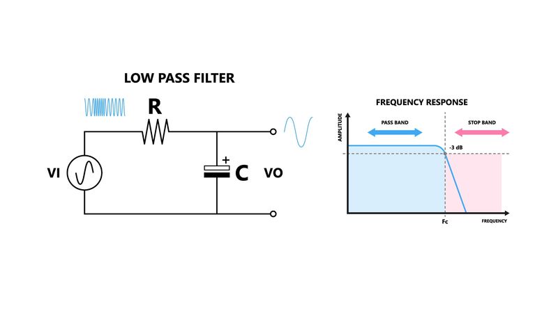
The low-pass filter (LPF) is a linear time-invariant (LTI) system that allows low-frequency signals to pass while attenuating higher-frequency components. The transition between the passband and stopband is characterized by the cutoff frequency (fc).
The cutoff frequency is defined at the point where the magnitude of the transfer function falls to 0.707 of its zero-frequency value, corresponding to a –3 dB reduction in amplitude. [1] On a Bode magnitude plot (gain vs. logarithmic frequency), a first-order low-pass filter exhibits a slope of –20 dB per decade beyond the cutoff frequency. The second-order filter rolls off at –40 dB/decade, while an nth-order design shows a –20n dB/decade roll-off, depending on the filter design and topology.
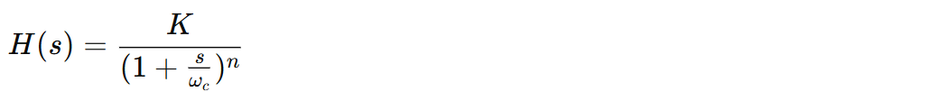
The general transfer function of a continuous-time low-pass filter is expressed as:
In discrete‑time implementations, the transfer function is expressed in the z‑domain as H(z), as discussed later.
Time-Domain Interpretation
In the time domain, a low-pass filter acts as a smoothing circuit. Once a square-wave input signal passes through an RC low-pass filter circuit, the output signal becomes rounded because the circuit integrates the rapid transitions.
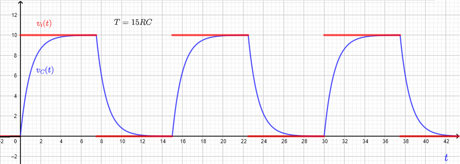
Essentially, the capacitor and resistor combination behaves as an integrator for high-frequency signals, suppressing sharp edges and reducing transient noise. This property is crucial for cleaning noisy analog waveforms, stabilizing sensor outputs, and improving signal quality in both analog and digital systems.
Passband, Stopband and Attenuation
Passband: Frequencies below the cutoff frequency, where the signal experiences minimal attenuation and the amplitude response remains nearly constant.
Transition Band: The frequency range around the cutoff frequency where the amplitude decreases from the passband to the stopband level. The steepness of this transition depends on the filter order and response type (e.g., Butterworth, Bessel, or Chebyshev).
Stopband: Frequencies above the transition region where the low-pass filter strongly attenuates the signal, ideally approaching zero gain.
Amplitude and Phase Response
The amplitude response of a low-pass filter defines how much each frequency component is reduced, while the phase response describes the phase shift introduced at each frequency.
In audio signal processing, instrumentation, and communication systems, maintaining linear phase response is vital. Bessel filters and certain FIR (Finite Impulse Response) digital filters exhibit nearly constant group delay, preserving the original waveform shape. In contrast, filters with nonlinear phase—such as Chebyshev or Butterworth—may introduce phase distortion or ringing, which can degrade the integrity of the output signal in sensitive applications.
Recommended Reading: Low Pass Filter vs High Pass Filter – Theory, Design, and Applications
Analog Low‑Pass Filters
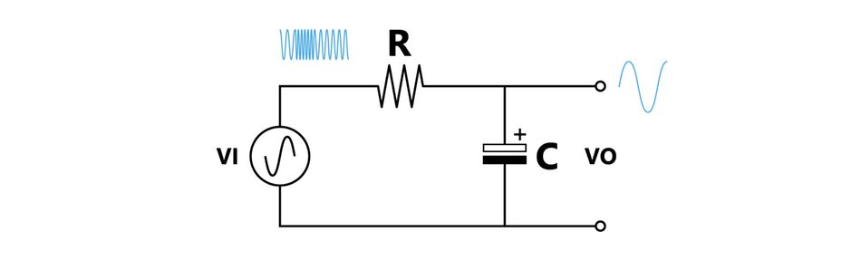
Passive RC Low‑Pass Filter
The most fundamental low-pass filter circuit consists of a resistor (R) and a capacitor (C) connected in series, with the output signal taken across the capacitor. The capacitive reactance (Xc):
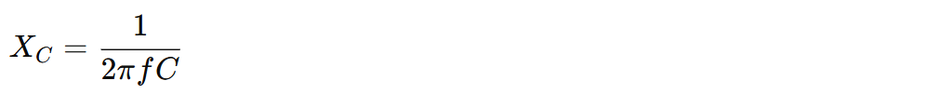
is large at low frequencies, so most of the input signal voltage appears across the capacitor. Xc becomes small at the high frequencies, the capacitor effectively shorts the output, and high-frequency signals are attenuated.
The cutoff frequency (fc) is given by:

Once the frequency equals the cutoff frequency, the output amplitude drops to approximately 70.7% of the input (–3 dB), and the phase shift equals –45° for a first-order RC low-pass filter. Because no external energy source is used, passive filters have a maximum gain of unity.
Cascading multiple RC sections increases the filter order, producing a steeper roll-off (–40 dB/decade for a second-order filter). [2] However, a slight increase in the cascading factor slightly lowers the combined cutoff frequency, so designers must adjust component values to maintain the desired frequency response.
Passive RL Low‑Pass Filter
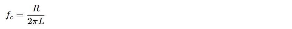
The passive RL low-pass filter employs a resistor (R) and an inductor (L) in series, with the output taken across the resistor. The inductive reactance is given by:

which increases with frequency. This implies that, at lower frequencies, the inductive reactance is small, so most of the voltage drops across the resistor. At high frequencies, the inductive reactance becomes large, most of the voltage drops across the inductor, and the output is attenuated.
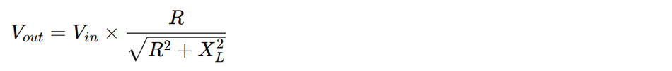
The cutoff frequency (fc) occurs when Inductive Reactance = Resistance:
The output voltage magnitude is:
Cascading RL stages increases the order and improves attenuation, but as with RC networks, the actual -3 dB point shifts slightly due to loading effects.
Active Low‑Pass Filters
Passive filters are limited by loading and unity-gain issues, while active filters overcome these limitations using operational amplifiers (op-amps) or transistor stages with frequency-selective feedback. These active filters can provide gain, precise cutoff frequency control, and sharper bandwidth shaping.
The two common filter design architectures are:
1. Sallen–Key Topology
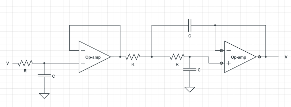
Utilizes a unity-gain buffer or amplifier to isolate the RC network from the load. It offers simplicity, predictable response, and good stability for low- to mid-frequency applications, though the op-amp bandwidth limits performance.
2. Multiple-Feedback (MFB) Topology
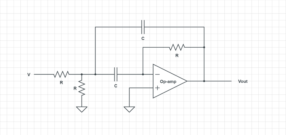
Incorporates reactive components in both feedback and input paths. It provides improved high-frequency performance and Q-factor control but requires careful component tolerance matching.
Standard Second-Order Active Low-Pass Transfer Function
The general second‑order low‑pass transfer function is written as
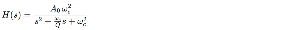
Adjusting Q modifies amplitude behavior near the cutoff frequency, determining whether the response is Butterworth, Bessel, or Chebyshev. The component values in the Sallen–Key or MFB network set both ωc and Q.
Filter Response Types
Different types of filters balance flatness, group delay, and stopband attenuation. Selecting the right low-pass filter response ensures optimal performance for the intended application. Let’s go through the comparison below:
| Filter Type | Characteristics | Applications |
| Butterworth | Maximally flat amplitude in the passband, no ripple, monotonic roll-off (–20n dB/decade) | Audio, instrumentation, anti-aliasing, and equalizers requiring smooth response |
| Bessel | Flat group delay and linear phase response, slower attenuation | Time-domain critical systems (pulse, data communications) with minimal waveform distortion |
| Chebyshev Type I | Sharper transition, equiripple passband, monotonic stopband | Applications tolerating passband ripple but needing steep roll-off, such as communications |
| Chebyshev Type II | Flat passband, equiripple stopband, moderate slope | Cases needing excellent stopband attenuation with ripple-free passband |
| Elliptic (Cauer) | Ripple in both bands; steepest slope for given order | Highly selective systems where stopband attenuation is critical |
Butterworth filters are a popular default because they provide maximum flatness in the passband. Bessel filters preserve waveform shape due to their constant group delay, making them suitable for analog communication systems. Chebyshev & elliptic filters achieve steeper roll‑off at the cost of ripple and more complex implementations.
Design Example: Passive RC Low‑Pass Filter
Suppose you need to limit noise above 1 kHz from a sensor signal. Choosing R=1.59 kΩ and C=100 nF yields:

The Bode plot will show a flat passband below 1 kHz and a –20 dB/decade roll-off above it. Cascading two identical RC sections yields a –40 dB/decade slope but shifts the –3 dB point slightly lower. It is better to use capacitors and resistors with tight tolerances to maintain the desired cutoff frequency and consistent filter performance.
Recommended Reading: Difference between Active and Passive Filters?
Digital Low‑Pass Filters
Discrete-Time Representation
In digital signal processing (DSP), signals exist as discrete sequences of samples. A digital low-pass filter (LPF) operates on these samples to suppress high-frequency electronic components while preserving low-frequency signals.
The ideal low-pass filter has an infinitely long impulse response, which is impossible to realize in practice. Therefore, digital filters approximate it using either infinite impulse response (IIR) or finite impulse response (FIR) structures, depending on system requirements such as phase linearity, stability, and computational cost.
IIR vs FIR Filters
Infinite impulse response (IIR) filters are recursive; they compute each output sample using both current and past inputs and past outputs. The simple first‑order IIR low‑pass filter, an exponential moving average, can be described by the difference equation:


Smaller α provides more substantial attenuation of high-frequency noise but introduces greater phase delay. This simple algorithm is widely used in microcontrollers, sensors, and audio processing, where computational efficiency is critical.
IIR filters can replicate analog filter responses such as Butterworth, Chebyshev, or Bessel with fewer coefficients than FIR filters, making them ideal for constrained systems. [3] However, IIR filters exhibit nonlinear phase and must be carefully designed to ensure stability—poles must lie inside the unit circle in the z-plane to guarantee BIBO stability.
Finite impulse response (FIR) filters compute outputs solely from current and past input samples, making them inherently stable and capable of exact linear‑phase responses. However, achieving a sharp transition band requires many coefficients, increasing computational load and latency. FIR filters are standard in applications where linear phase and stability are paramount and memory resources are available.
Designing Digital Low-Pass Filters via Analog Prototypes
The common method for designing IIR filters is to create an analog prototype (e.g., a Butterworth or Chebyshev filter) and then transform it into a digital filter. Two primary discretisation techniques exist:
1. Impulse‑Invariant Transformation (IIT): Directly samples the analog impulse response. It is simple but may introduce aliasing, as high-frequency components of the analog response fold into the digital passband.
2. Bilinear Transform (BT): Maps the analog transfer function Ha(s) from the s‑plane to a digital transfer function Hd(z) by substituting:

where T=1/fs is the sampling interval. The bilinear transform maps the analog jω-axis onto the unit circle in the z-plane, preserving stability by ensuring that poles in the left half of the s-plane map inside the unit circle.
However, this mapping is nonlinear, causing frequency warping, equal frequency steps in the digital domain correspond to unequal steps in the analog domain. To correct this, designers apply prewarping so the digital cutoff frequency aligns precisely with the desired value:

where ωa0 and ωd0 are the analog and digital cutoff angular frequencies, respectively. This ensures accurate frequency-response matching between the analog prototype and its digital counterpart.
FIR Filter Design Methods
While the bilinear transform is ideal for IIR filters, FIR filter design typically uses windowing or frequency-sampling techniques.
The window method begins with the ideal infinite impulse response (a sinc function) of an ideal low-pass filter, which is truncated by a window function (e.g., Hamming, Hanning, or Blackman). The choice of window controls ripple amplitude, transition bandwidth, and stopband attenuation.
Software tools such as MATLAB and Python’s SciPy provide functions like firwin() and remez() for automated FIR filter synthesis. These filters are often employed in multi-rate processing, interpolation, decimation, and real-time DSP applications requiring linear phase and consistent bandwidth characteristics.
Real‑World Applications of Low‑Pass Filters
Low‑pass filters are ubiquitous in electrical and electronic systems. The following list summarises major application areas:
Audio Processing
Speaker Crossovers: LPFs route low-frequency signals to subwoofers, while high-pass filters direct higher frequencies to tweeters, ensuring optimal energy distribution and balanced sound.
Equalization and Tone Control: Adjust amplitude balance between bass and treble by filtering unwanted high-frequency signals.
Subwoofer Integration: Maintain smooth frequency response between subwoofers and main speakers by matching cutoff frequency and phase alignment.
Noise Reduction: Remove hiss and unwanted high-frequency content in audio recordings for cleaner playback and recording fidelity.
Radio Communications
Channel Filtering: Low-pass filters and band-pass filters isolate desired communication channels while rejecting adjacent interference.
Bandwidth Limitation: Restrict transmission to a defined range of frequencies, ensuring compliance with communication standards and minimizing spectral leakage.
Intermediate-Frequency (IF) Processing: Used in superheterodyne receivers to select and amplify the desired IF signal while suppressing unwanted sidebands.
Demodulation: Recover baseband information by removing the high-frequency carrier components from modulated signals.
Power Supplies and EMI Suppression
Ripple Reduction: In DC power supplies, low-pass filters smooth rectified outputs by attenuating AC ripple.
EMI Filtering: Suppress high-frequency noise generated by switching devices or nearby circuits, improving system signal integrity and electromagnetic compatibility.
Digital Signal Smoothing
Anti-Aliasing Before ADC: Analog low-pass filters limit input bandwidth to below half the sampling rate (Nyquist frequency). Steep roll-off designs—such as Butterworth, Chebyshev, or Bessel—ensure sufficient attenuation of out-of-band frequencies before digital conversion.
Data Smoothing: Digital LPFs clean noisy sensor data, stabilize control loop feedback, and prepare signals for real-time decision-making in automation and robotics.
Image Processing: In digital imaging, LPFs act as blurring filters to suppress noise, reduce aliasing during down-sampling, and enhance subsequent edge detection.
Biomedical Engineering
Physiological Signal Filtering: Remove high-frequency interference from EMG, ECG, and EEG signals while retaining diagnostically relevant low-frequency components.
Signal Conditioning: Prepare biosignals for analog-to-digital conversion or algorithmic analysis.
Medical Imaging: Apply low-pass filtering to reduce speckle noise, smooth contours, and enhance overall image quality in modalities such as MRI and ultrasound.
Miscellaneous and Industrial Applications
Touchscreens and Control Systems: Smooth analog input variations, minimizing jitter and ensuring stable response.
Camera Stabilization and Motion Sensors: LPFs in feedback control loops reduce high-frequency oscillations, improving precision and damping mechanical resonance.
Automotive Electronics: Filter sensor outputs in engine management, braking, and safety systems to eliminate electrical noise and enhance reliability.
Low-pass filters remain useful in both hardware and software implementations, from simple RC circuits to advanced DSP algorithms. Their ability to balance attenuation, phase response, and bandwidth control makes them a cornerstone of modern signal-processing and system-design practices.
Recommended Reading: BAW filters for Performance Improvements in Wi-Fi, 5G, and RF Applications
Design Guidelines and Practical Considerations
Successfully designing a low‑pass filter requires balancing theoretical considerations with practical constraints.
Selecting the Cutoff Frequency
- Identify the Highest Frequency of Interest: In audio processing, this may be the upper bound of audible content; in anti‑aliasing, it is half the sampling rate.
- Allow Margin for Transition: Real filters have a finite roll‑off. When designing an anti‑aliasing filter, sample rates 5–10 times the desired signal bandwidth yield realistic transition bands.
- Consider System Noise and Interference: Choose cutoff frequency (fc) low enough to suppress noise but high enough not to distort the desired signal.
Choosing Filter Order and Type
Order: Higher order increases roll‑off steepness (20 dB/decade per order) but also increases component count (analog) or computational complexity (digital). For simple noise reduction, a first‑ or second‑order filter is often sufficient. For anti‑aliasing or communications channels, higher orders (4th–8th) may be required.
Filter Type: Decide among Butterworth (flat amplitude), Bessel (constant group delay), Chebyshev (steep roll‑off with ripple), or elliptic (steepest). Use design tables or software (e.g., TI FilterPro, MATLAB, Python).
Active vs Passive: Passive RC or RL filters are suitable for high‑frequency or power applications and require no supply. Active filters provide gain and are better for low‑frequency precision filtering, but require power supplies and op‑amp bandwidth considerations.
Component Selection
Resistor and Capacitor Tolerances: Tight tolerances (1% or better) reduce cutoff frequency variations. Use low‑noise film capacitors or polypropylene types for audio.
Inductor Considerations: Inductors introduce series resistance and parasitic capacitance; choose high‑quality inductors for RF or audio applications.
Op‑Amp Selection: For active filters, select op‑amps with unity‑gain bandwidth at least an order of magnitude higher than the cutoff frequency to avoid phase shift and gain peaking. Ensure adequate slew rate and low noise.
Digital Implementation Considerations
Sampling Rate: Ensure the sampling frequency is sufficiently high (e.g., >2× the highest filtered frequency) and ideally 5–10× for comfortable anti‑aliasing transition.
Fixed‑Point vs Floating‑Point: In microcontrollers, fixed‑point arithmetic saves resources but requires careful scaling to maintain precision and avoid overflow.
Coefficient Quantisation: Quantisation of filter coefficients may affect frequency response. Use higher precision for narrowband or high‑order filters.
Latency: IIR filters have lower latency compared to FIR filters for a given transition width. For real‑time control, prefer low-latency filters; for offline processing, FIR filters may be acceptable.
Design Workflow
- Define Specifications: Determine the desired cutoff frequency, passband ripple and stopband attenuation.
- Choose Filter Response and Order: Select Butterworth, Chebyshev, etc., and decide the filter order based on roll‑off requirements.
- Select Implementation: Decide on passive, active or digital. For digital, choose IIR or FIR.
- Compute Component Values or Coefficients: Use standard design equations for RC/RL filters, design tables for active filters or software for digital filters.
- Prototype and Simulate: Use circuit simulation (SPICE) or DSP tools (MATLAB/Python) to validate the frequency response. [4] You can adjust values if necessary.
- Build and Test: Implement the filter on a breadboard, PCB or microcontroller. Measure the response with an oscilloscope or network analyser to ensure it meets specifications. Iterate as needed.
Visualizing the Frequency Response
The following conceptual diagram illustrates a typical low‑pass filter frequency response. The passband is flat until the cutoff frequency (fc); at the cutoff, the magnitude drops by 3 dB, and beyond fc, the amplitude decreases with a constant slope.

Idealised magnitude response of a low‑pass filter with passband, −3 dB cutoff, and stopband. Real filters have finite transition bands and may exhibit ripple or non‑linear phase.
Recommended Reading: Selecting the Best Power Solution for Radio Frequency Signal Chain Phase Noise Performance
Conclusion
Low‑pass filters are foundational components of electronic and digital systems. They define what frequency content is allowed to pass through circuits and algorithms, thereby shaping audio, controlling sensor signals and preventing aliasing in digital conversion. From simple RC or RL networks to sophisticated active or digital filters, the underlying principle is to attenuate frequencies above a chosen cutoff. Understanding the trade‑offs between filter orders, responses (Butterworth, Bessel, Chebyshev, elliptic), and analog versus digital implementations is essential for engineering success.
Future developments include integrated digital filters in microcontrollers and system‑on‑chip solutions that offer configurable cutoff frequencies and orders. With the continuous increase in bandwidths and sampling rates, careful filter design will remain a critical skill for digital design engineers, hardware developers and electronics students.
Frequently Asked Questions (FAQ)
1. What is a low‑pass filter and what does it do?
A. A low‑pass filter allows low‑frequency signals to pass while attenuating high‑frequency signals. The transition between passband and stopband is defined by the cutoff frequency (–3 dB point). LPFs are used to remove high‑frequency noise, prevent aliasing and isolate desired signal components.
2. What is the difference between Butterworth and Chebyshev low‑pass filters?
A. Butterworth filters have a maximally flat passband with no ripple but moderate roll‑off. Chebyshev filters (Type I and II) have passband or stopband ripple but exhibit steeper roll‑off, allowing a narrower transition band. Tutorials often show how to choose between flatness and selectivity based on your desired bandwidth and attenuation.
3. When should I use an active low‑pass filter instead of a passive one?
A. Use active filters with op-amps for precision and gain in low-frequency applications. Choose passive RC filters for DIY or Arduino circuits handling high-power or ohm-level impedance signals without external power.
4. How do digital low‑pass filters differ from analog ones?
A. Digital filters process discrete samples via algorithms, allowing precise tuning and software control. Analog filters use resistors, capacitors, and inductors, offering instant response without latency, ideal for Arduino hardware and sensor tutorials.
5. What is anti‑aliasing and why are low‑pass filters used for it?
A. Anti-aliasing low-pass filters block frequencies above half the sampling rate to prevent aliasing distortion. Their decibel roll-off ensures clean signal conversion with minimal high-frequency attenuation in digital recording and sensor interfaces.
6. Can I implement a low‑pass filter using software only?
A. Yes. Software-based digital filters (IIR or FIR) run easily on Arduino, Raspberry Pi, or microcontrollers. Numerous tutorials demonstrate coding low-pass filter algorithms to control cutoff frequency and filter strength dynamically.
References
[1] Electronic Tutorials. Frequency Response Analysis of Amplifiers and Filters [Cited 2025 October 21] Available at: Link
[2] GWU. "Chapter 16 - Active Filter Design Techniques" [Cited 2025 October 21] Available at: Link
[3] ResearchGate. Design and Comparison Between IIR Butterworth and Chebyshev Digital Filters using MATLAB [Cited 2025 October 21] Available at: Link
[4] MATLAB. Frequency Response Estimation Using Simulation-Based Techniques [Cited 2025 October 21] Available at: Link