Source Transformation: Theory, Methods, and Practical Implementations for Modern Electronics and Digital Design
Source transformation is the method of converting a voltage source with series resistance into an equivalent current source with parallel resistance (and vice versa). This guide explains the theory, math, circuit examples, and practical applications for modern digital and hardware engineers.

03 Dec, 2025. 20 minutes read
Key Takeaways
Fundamental technique – Source transformation converts a voltage source in series with a resistor into an equivalent current source in parallel with the same resistor (and vice-versa) while preserving all external circuit behavior.
Theoretical basis – The method is grounded in Ohm’s law and the Thévenin–Norton equivalence. A Thévenin model uses a voltage source and series resistance, whereas a Norton model uses a current source and parallel resistance.
Versatile application – Effective for linear DC and AC circuits, including those involving complex impedances. It also extends to digital hardware for termination networks, I/O buffer modeling, output-driver characterization, and power-distribution analysis.
Simplification and analysis – Converting between source forms enables easier combination of sources, reduces the number of mesh or nodal equations, supports faster simulation, and improves design optimization during PCB and hardware-system development.
Cautions and limitations – Valid only when a pure source–resistor pair exists. Engineers must maintain correct polarity and orientation, and apply special care when dealing with dependent sources, reactive components, and non-linear devices.
Introduction
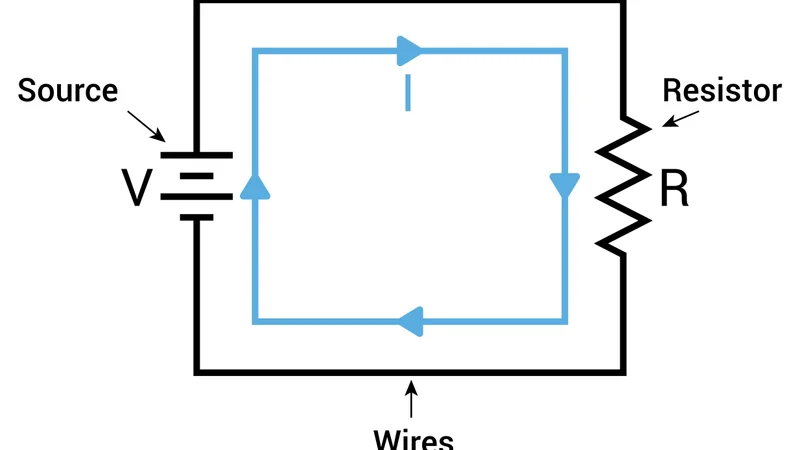
Electrical and electronic systems—from simple resistive networks to high-speed digital hardware—fundamentally depend on controlled delivery of energy from voltage and current sources. During circuit analysis or hardware design, complex networks often need to be reduced without altering how they behave at their terminals. Source transformation provides a rigorous method for achieving this simplification by converting a voltage source in series with a resistor into an equivalent current source in parallel with the same resistor, and vice versa. This equivalence enables circuit blocks to be expressed in whichever form is most convenient for analysis, allowing for faster combination of sources, clearer insight into power flow, and more efficient modeling of real-world components.
The method is grounded in Thévenin’s and Norton’s theorems, which state that any linear circuit containing independent sources and resistances can be reduced to either a voltage-source–series-resistance model or a current-source–parallel-resistance model. These dual forms, linked directly through Ohm’s law, establish the mathematical basis that permits seamless conversion between the two. Because many practical components—regulators, output drivers, bias networks, and termination structures—naturally behave like ideal sources with internal resistance, source transformation becomes an essential tool for accurately representing their behavior. Its usefulness extends into AC analysis with phasors and complex impedances, small-signal modelling of transistor stages, and optimisation of power-delivery paths on modern PCB layouts.
This article outlines the theory behind source transformation and explains how to perform voltage-to-current and current-to-voltage conversions. Key applications, practical tips, and limitations are also summarised for quick reference.
Fundamentals of Sources and Equivalence
Understanding how voltage and current sources operate is crucial for efficient circuit analysis and hardware design. This knowledge forms the foundation for applying Thévenin and Norton equivalence, enabling engineers to simplify networks, optimize PCB layouts, and model real-world component behavior accurately.
Voltage and Current Sources
Electrical sources are the fundamental building blocks of circuits, delivering controlled energy to loads. They are classified into two main types:
Voltage sources maintain a constant voltage across their terminals, independent of the current drawn. Ideal voltage sources have zero internal resistance, while practical sources, such as batteries or DC power supplies, include a series resistance to model real-world losses. Understanding voltage source behavior is essential for circuit analysis, PCB power distribution, and signal integrity design.
Current sources provide a constant current regardless of the voltage across their terminals. Ideal current sources have infinite parallel resistance. Practical implementations often use transistor-based circuits or active current mirrors. Mastery of current sources supports load analysis, bias network design, and high-speed hardware applications.
Sources can be independent, with fixed values, or dependent, where the source value is controlled by another voltage or current elsewhere in the circuit. Independent sources are straightforward to transform using standard source transformation techniques, whereas dependent sources require careful attention to ensure that the controlling variable remains consistent throughout any conversion.
Thévenin and Norton Equivalents
Thévenin and Norton theorems form the theoretical backbone of source transformation, enabling engineers to simplify complex circuits into manageable models for analysis and design.
Thévenin Equivalent: Any linear circuit with independent sources and resistances can be represented as a single voltage source Vth in series with a resistor Rth. The open-circuit voltage at the terminals equals Vth, and the short-circuit current is Isc = Vth / Rth. This representation is especially useful for voltage analysis, load calculations, and PCB power path optimization.
Norton Equivalent: The same circuit can be expressed as a current source (In) in parallel with a resistor Rn. The conversion relationships are:
In = Vth / Rth
Vth = In * Rn
Rn = Rth
Norton equivalents are particularly effective for current distribution analysis, parallel load modelling, and driver circuit design.
Both equivalents produce identical terminal behavior, allowing them to be interchanged seamlessly in linear circuits. Source transformation applies these equivalences locally, converting a voltage source with its series resistor into a current source with a parallel resistor—or vice versa—without changing the behavior observed by external components. This approach simplifies circuit simulation, reduces mesh and nodal equations, and improves system-level design clarity.
| Equivalent Form | Description | Mathematical Relationship |
| Thévenin Equivalent | Voltage source Vth in series with resistor Rth | Open-circuit voltage: V_oc = VthShort-circuit current: I_sc = Vth / Rth |
| Norton Equivalent | Current source (In) in parallel with resistor Rn | Open-circuit voltage: V_oc = In * RnShort-circuit current: I_sc = In |
In source transformation, we convert between these equivalents while maintaining the same iii–vvv characteristic. In practice, we rarely need to derive the Thévenin or Norton equivalent of a complex network; instead, we perform local conversions between a source and its series or parallel resistor.
Ohm’s Law and Linearity
Source transformation relies on the fundamental principles of Ohm’s law and the linearity of resistive circuits. Understanding these principles ensures that voltage-to-current and current-to-voltage conversions preserve the behavior seen by the rest of the circuit.
Ohm’s Law defines the relationship between voltage, current, and resistance:
V = I * R
I = V / R
R = V / I
This applies to resistors in both series and parallel configurations, as well as to the resistor in a source–resistor pair during transformation.Linearity means that the superposition principle holds: the response of a linear circuit to multiple sources is the sum of the responses to each source individually. This property allows engineers to convert sources without affecting the external voltage–current relationship.
During a source transformation:
The resistor value remains unchanged.
The product of the source value and the resistor is constant:
For voltage-to-current conversion: I_s = V_s / R
For current-to-voltage conversion: V_s = I_s * R
Because of linearity, the open-circuit voltage and short-circuit current at the terminals remain identical, ensuring the transformed source behaves equivalently to the original.
Recommended reading: Open Circuit vs Short Circuit: Core Differences between Open and Closed Circuit
Source Transformation Fundamentals
What is Source Transformation?
Source transformation is a fundamental technique in electrical and electronics engineering that converts a practical voltage source—an ideal voltage source in series with a resistor—into an equivalent current source in parallel with the same resistor, or vice versa, while preserving the terminal voltage–current relationship. This technique is widely applied in circuit analysis, linear DC and AC networks, and digital hardware design to simplify complex circuits, reduce computational effort, and enable efficient simulation.
The transformation is valid only under these conditions:
The resistor must be directly in series with the voltage source or in parallel with the current source.
No additional circuit elements should intervene between the source and the resistor.
The circuit must be linear and time-invariant, ensuring predictable superposition and proportionality.
Key conversion formulas:
Voltage-to-current transformation:
Is = Vs / RCurrent-to-voltage transformation:
Vs = Is × R
These formulas ensure that the external circuit behavior, including the open-circuit voltage and short-circuit current, remains unchanged. This property is crucial when analyzing circuits for load conditions, power distribution, or signal integrity.
Theoretical Derivation
Consider a voltage source Vs in series with a resistor R:
Short-circuit analysis:
When the terminals are shorted, the current through the short is:
Isc = Vs / ROpen-circuit analysis:
When the terminals are open, the voltage across the terminals is:
Voc = Vs
For the equivalent current source (Is) in parallel with the same resistor R:
Short-circuit current: Isc = Is
Open-circuit voltage: Voc = Is × R
By setting Is = Vs / R and Vs = Is × R, it is confirmed that both the terminal voltage and current remain identical in the original and transformed configurations.
This derivation demonstrates that source transformation preserves external circuit behavior, making it a reliable tool for:
Simplifying mesh and nodal analysis.
Combining multiple voltage or current sources efficiently.
Modeling real-world components like resistive power sources, digital driver outputs, and termination networks.
Facilitating simulation in SPICE and other circuit design software.
By mastering source transformation, engineers and electronics students can analyze complex networks, including mixed-source DC circuits, phasor-domain AC circuits, and high-speed digital signal paths, with greater precision and confidence.
Recommended reading: DC to AC Inverter Circuits – Theory, Design and Practical Implementation
Step-by-Step Source Transformation Procedure
Source transformation becomes straightforward when approached systematically. Following a structured method ensures accuracy in voltage-to-current or current-to-voltage conversions and reduces errors in circuit analysis.
1. Identify the Source–Resistor Pair
Locate a practical voltage source in series with a resistor or a current source in parallel with a resistor. Ensure no other elements intervene between the source and resistor. Only pure source–resistor pairs are eligible for direct transformation in linear circuits.
2. Calculate the Equivalent Source
For a voltage source Vs in series with R:
Equivalent current source Is = Vs / RFor a current source Is in parallel with R:
Equivalent voltage source Vs = Is * R
These calculations preserve terminal voltage, short-circuit current, and load behavior, essential for accurate electronic circuit design and simulation.
3. Maintain Polarity and Direction
Correct orientation is critical. Align the current source arrow with the positive terminal of the voltage source, and preserve the resistor’s position relative to the source. Incorrect polarity can reverse currents and produce erroneous results, especially in mixed-source networks.
4. Replace the Original Pair
Remove the source–resistor pair and replace it with the equivalent configuration:
Voltage source → series resistor
Current source → parallel resistor
This step converts the network while keeping external node behavior identical.
5. Simplify and Combine Sources
After transformation, combine series voltage sources or parallel current sources where possible. Similarly, combine resistors in series or parallel to reduce the overall network complexity. This step streamlines mesh analysis, nodal analysis, and SPICE simulations, especially in complex DC and AC circuits.
Conditions and Limitations of Source Transformation
While source transformation is a powerful technique for circuit simplification and electronic analysis, it must be applied under specific conditions to ensure accurate results. Understanding these limitations is critical for engineers working with linear DC and AC circuits, digital hardware, or simulation environments.
1. Linearity Requirement
Source transformation is valid only in linear, time-invariant circuits. Non-linear components such as diodes, transistors in active regions, and semiconductor switches cannot be directly transformed. For circuits containing non-linear devices, alternative methods like nodal analysis, mesh analysis, or Laplace transform techniques are recommended.
2. Pure Source–Resistor Pair
The resistor must be the only element in series (for voltage sources) or parallel (for current sources). If other components lie between the source and resistor, the circuit must first be reorganized using series-parallel combinations or source shifting before performing a transformation.
3. Ideal Sources Limitation
An ideal voltage source with zero internal resistance or an ideal current source with infinite internal resistance cannot be transformed directly.
Practical sources must have a finite series or parallel resistance to allow a valid voltage-to-current or current-to-voltage conversion.
4. Dependent Sources
Dependent sources, whose values rely on a circuit variable elsewhere, require caution:
Transformation is possible only if the controlling variable is local to the source–resistor pair.
If the controlling variable exists elsewhere in the network, direct transformation may break the dependency and produce incorrect results. In such cases, it is safer to compute Thévenin or Norton equivalents of the network instead.
5. Polarity and Orientation
Maintaining correct polarity and direction is essential:
The current source arrow must align with the positive terminal of the corresponding voltage source.
Reversing orientation can lead to opposite current flow or incorrect voltage drops, compromising both DC and AC analysis.
6. AC Circuit Considerations
For AC circuits analyzed in the phasor domain:
Resistances are replaced with complex impedances (Z = R + jX).
Phase relationships must be preserved when transforming between voltage and current sources.
Non-linear or time-varying components, such as saturating inductors or variable capacitors, require more advanced methods beyond simple source transformation.
Applying Source Transformation to DC Circuits
Source transformation is particularly useful for simplifying DC circuits, where multiple sources and resistors make mesh or nodal analysis cumbersome. By converting voltage sources in series with resistors to current sources in parallel, or vice versa, engineers can streamline calculations, combine like sources, and reduce the number of equations needed for analysis.
Example: Simplifying a Mixed-Source Network
Consider a network containing a 1 A current source in parallel with a 10 Ω resistor, connected to a resistive bridge. Applying source transformation:
Convert the current source to a voltage source:
Vs = Is * R = 1 A * 10 Ω = 10 V
Resulting in a 10 V voltage source in series with a 10 Ω resistor.
Next, suppose a branch has a 10 V voltage source in series with a 5 Ω resistor:
Convert to a current source:
Is = Vs / R = 10 V / 5 Ω = 2 A
Similarly, a branch with a 15 Ω resistor in series with a 10 V source becomes:
Is = Vs / R = 10 V / 15 Ω ≈ 0.667 A
Once converted, parallel current sources can be combined algebraically, and series or parallel resistors simplified using:
Series: R_total = R1 + R2 + ...
Parallel: 1 / R_total = 1 / R1 + 1 / R2 + ...
After combining sources and resistors, Kirchhoff’s Voltage Law (KVL) or Kirchhoff’s Current Law (KCL) can be applied to compute currents or voltages across target components efficiently.
Recommended reading: KCL Circuit Analysis: Advanced Engineering Methods & Best Practices 2025

Source Shifting and Ideal Cases
In some networks, a source may not have an explicit series or parallel resistor (e.g., an ideal voltage source directly across nodes).
Source shifting repositions the source to introduce a resistor for valid transformation.
Ideal sources without finite resistance cannot be transformed.
Dependent Sources in DC Networks
Dependent sources must be handled carefully:
If the controlling variable lies within the source–resistor pair, transformation is possible. For example, a voltage-controlled voltage source in series with a resistor can be converted to a current source with:
Is = V_control / R
If the controlling variable is external, use Thévenin/Norton derivation rather than direct transformation to preserve circuit behavior.
Extending Source Transformation to AC Circuits
In AC circuit analysis, source transformation remains a powerful method for simplifying networks, but its application requires using phasors, complex impedances, and frequency-dependent relationships. By converting between AC voltage sources with series impedance and AC sources with parallel impedance, engineers can reduce circuit complexity, streamline nodal or mesh calculations, and model real-world components such as reactive loads, drivers, and termination networks.
AC source transformation applies the same principle as in DC circuits, but substitutes resistors with complex impedances (denoted as Z), ensuring that magnitude and phase are preserved.
Voltage-to-Current Transformation in AC Circuits
A sinusoidal voltage source in series with an impedance Z can be replaced by an equivalent current source in parallel with the same impedance.
Given:
Voltage source: Vs ∠θ
Series impedance: Z = R + jX
Equivalent current source:
Is = (Vs ∠θ) / Z
Orientation of the current source must align with the phase angle of the original voltage source.
Current-to-Voltage Transformation in AC Circuits
A sinusoidal current source in parallel with an impedance can be replaced by an equivalent voltage source in series with the same impedance.
Given:
Current source: Is ∠φ
Parallel impedance: Z = R + jX
Equivalent voltage source:
Vs = Is ∠φ * Z
Preserving Magnitude, Phase, and Impedance Behavior
Because AC circuits operate in the phasor domain, the transformation must preserve:
Magnitude (|V| and |I|)
Phase (θ, φ)
Impedance relationships (Z_total)
Failure to maintain phasor direction or complex impedance relationships can lead to incorrect amplitude or phase predictions in frequency-domain analysis.
Example: Transforming a Reactive AC Source
Consider a voltage source:
Vs = 12 ∠30°
Z = 8 + j6 Ω
Equivalent current source:
Is = 12 ∠30° / (8 + j6)
Or for a current source:
Is = 2 ∠–20°
Z = 4 – j3 Ω
Equivalent voltage source:
Vs = 2 ∠–20° * (4 – j3)
These calculations allow engineers to merge sources, simplify impedances, and perform accurate phasor-domain analysis in AC power systems, RF networks, analog circuits, and high-frequency PCB design.
Recommended Reading: Types of Circuits: A Comprehensive Guide for Engineering Professionals
Source Transformation in Digital and Hardware Design
Source transformation is not only a theoretical circuit-analysis tool—it is woven into the core of modern digital hardware engineering. From transmission-line terminations to driver modelling and power-delivery optimization, the ability to swap between Thévenin and Norton equivalents allows designers to simplify complex behaviour into predictable, simulation-friendly forms. This foundation becomes crucial as digital systems push into higher speeds, lower voltages, and denser architectures.
Recommended reading: Source Transformation in Electrical Circuit Analysis: Thevenin–Norton Equivalence & Circuit Simplification
Termination networks in high-speed digital circuits
High-speed digital signals propagate along PCB traces that behave as transmission lines once edge rates reach the sub-nanosecond range. At these speeds, even short traces exhibit characteristic impedance, and any mismatch between the driver, trace, and receiver causes reflections, ringing, overshoot, undershoot, and timing skew. Proper termination is therefore essential for signal integrity in high-speed digital design, DDR interfaces, microcontroller buses, and FPGA-level routing.
A common and effective technique is Thévenin termination, where two resistors—typically connected to the logic-high (VDD) and logic-low (GND) rails—form a resistor divider that matches the transmission-line impedance. If the two resistor values are R1 and R2, the effective Thévenin resistance that the line sees is:
R_th = (R1 × R2) / (R1 + R2)
For proper impedance matching in digital hardware, this equivalent resistance is chosen to satisfy:
R_th ≈ Z_0
where Z₀ is the characteristic impedance of the PCB trace (commonly 50 Ω, 60 Ω, or 75 Ω depending on stack-up and routing geometry).
Practical advantages of Thévenin termination
Improved signal integrity: Matching the impedance minimizes reflections, stabilizes voltage transitions, and reduces jitter and ringing on fast edges.
Reduced attenuation: Because the effective impedance matches the line, the load does not excessively dampen the signal even at very high frequencies.
Level shifting capability: By choosing R1 and R2 values, designers can intentionally bias the line, shifting the logic-high and logic-low thresholds for interfacing between devices with different I/O standards.
Deterministic timing: With reflections suppressed, propagation delay and rise/fall times remain predictable—critical for synchronous digital buses.
Design considerations and limitations
Higher power consumption: Thévenin termination continuously draws current through the divider network, increasing static power, significant in low-power or battery-based systems.
Increased board area: Two resistors are required per signal, which scales poorly for wide parallel buses.
Voltage-swing reduction: Biasing the line modifies the high-level and low-level voltages, which must remain compliant with the receiver’s input thresholds.
Relevance to source transformation
Digital output drivers—such as CMOS buffers—are frequently modeled as Thévenin equivalents: a voltage source (equal to VDD or VOH) in series with an output resistance R_out determined by MOSFET on-resistance. In many analyses, converting this to a Norton equivalent simplifies current-flow calculations, especially when modeling multiple drivers or termination networks.
The conversions follow directly from source-transformation theory:
From Thévenin to Norton:
I_N = V_th / R_thFrom Norton to Thévenin:
V_th = I_N × R_th
This duality allows engineers to select whichever representation yields simpler mathematical or simulation models when evaluating transmission-line behaviour, load interaction, or driver strength.
Recommended reading: Vdd vs Vss: Key Technical Differences and Implications in Electronics
Modeling output drivers and load interfaces
Modern digital output pins—whether from microcontrollers, FPGAs, ASICs, or high-speed transceivers—must drive loads that vary widely in resistance, capacitance, and topology. To evaluate voltage droop, output-current capability, timing behaviour, and signal integrity, engineers commonly represent an output stage using a Thévenin equivalent model. This abstraction captures the essential behaviour of a driver without requiring transistor-level detail.
In a typical CMOS output stage, the PMOS and NMOS transistors present a finite on-resistance. When the driver outputs a logic high, the PMOS on-resistance forms an effective output impedance R_out, and the output node behaves like a voltage source equal to V_DD in series with R_out. The Thévenin model, therefore, becomes:
V_th = V_DD
R_th = R_out
When driving an external load R_L, the resulting load voltage is determined by a simple voltage-divider relationship:
V_L = V_th × (R_L / (R_th + R_L))
This expression is fundamental for assessing whether the driver can meet VIH and VIL thresholds under worst-case loading, especially in power-constrained or high-fan-out systems.
Converting to a Norton model
If the analysis focuses on current flow—common in multi-load distribution networks, shared buses, or pull-down terminations—the Thévenin representation can be transformed into a Norton equivalent:
I_N = V_th / R_th
R_N = R_th
This Norton model expresses the output driver as a current source in parallel with an equivalent resistance, making it easier to compute how current splits between multiple loads or termination networks. This approach is widely used in:
bus-driver analysis,
chip-to-chip interface design,
multi-drop memory lines, and
current-budget estimation in dense digital circuitry.
Enhanced modelling for capacitive and mixed loads
Real digital loads are often not purely resistive. PCB traces introduce distributed capacitance and inductance, package pins introduce parasitic inductance, and device inputs include ESD structures and leakage paths. Engineers often extend the Thévenin or Norton model with additional components such as:
C_L for input capacitance,
L_pkg for package inductance,
R_leak for input-leakage paths,
C_trace and L_trace for transmission-line segments.
These extended models improve accuracy for rise-time prediction, overshoot modelling, and timing-budget analysis in high-speed digital hardware.
Why source transformation matters here
Source transformation—switching between voltage-source and current-source representations—allows designers to choose the model that provides the most transparent insight. Voltage-oriented analysis simplifies logic-level evaluation, while current-oriented analysis exposes how loads interact in complex digital interconnects. Both representations ultimately describe the same output stage, but each highlights different aspects of signal integrity, driver strength, and power delivery.
Digital twins and system modelling
As electronic systems become increasingly complex, digital twins have become essential tools for predictive analysis, performance optimization, and real-time monitoring. A digital twin replicates the behaviour of a physical electrical subsystem—such as a battery pack, power-delivery network (PDN), motor drive, or high-speed interface—inside a simulation environment. To ensure accurate yet computationally efficient simulations, these models frequently rely on Thévenin and Norton equivalents of internal circuit blocks.
Simplified Thévenin equivalents commonly represent power supplies, battery modules, and embedded regulators:
V_th — the open-circuit or nominal output voltage
R_th — the effective output impedance capturing wiring resistance, switching losses, and control-loop dynamics
This abstraction enables the digital twin to predict load regulation, transient response, voltage droop, and current distribution without simulating every passive component, switching node, or control element. When current-flow analysis or parallel-load estimation is required, the Thévenin representation can be converted to its Norton counterpart:
I_N = V_th / R_th
R_N = R_th
This Norton model is especially valuable for evaluating load sharing among multiple power sources, estimating peak current demand during state transitions, and analyzing short-circuit or stall conditions in electromechanical systems.
Recommended Reading: Digital Twins bridge the gap between product development and product operations
Application in large-scale systems
Digital twins used in data centres, industrial controllers, electric vehicles, and IoT networks rely on equivalent source models to simulate:
power-delivery networks (PDNs) across multilayer PCBs,
dynamic voltage scaling (DVS) behaviour in processors,
motor-drive response under varying torque and speed profiles,
battery state-of-charge (SOC) and state-of-health (SOH) estimation,
system-level EMI and transient suppression,
thermal-electrical interactions in high-density electronics.
Because these environments involve thousands of interacting nodes, using Thévenin/Norton models dramatically reduces computational load while preserving accuracy where it matters—at the interfaces.
Why source transformation is critical in digital-twin workflows
Source transformation ensures that engineers can switch between voltage-oriented and current-oriented perspectives depending on the simulation goal. For example:
Voltage-based models simplify transient response and load-regulation analysis.
Current-based models improve accuracy for power-sharing, parallel-supply distribution, and fault modelling.
Switching between forms allows optimisation of simulation runtime without sacrificing insight.
This flexibility makes source transformation a foundational modelling technique inside modern digital-twin platforms used by power-electronics engineers, system architects, and hardware verification teams.
SPICE and simulation practice
Circuit-simulation tools such as SPICE, LTspice, PSpice, and Spectre implement source transformation internally to speed up matrix solving, improve convergence, and reduce simulation overhead. Although the transformation is often hidden behind the solver algorithms, understanding how Thévenin and Norton equivalents are applied allows hardware engineers to interpret waveforms, detect modelling errors, and build more robust simulation environments.
Many SPICE-level component models—particularly those for voltage regulators, op-amps, logic output stages, and sensor interfaces—are provided in a simplified Thévenin or Norton form. For example, a device datasheet may specify:
open-circuit output voltage (V_th)
output impedance (R_th)
short-circuit output current (I_SC)
Because these parameters map directly to Thévenin and Norton equivalents, designers can quickly verify model accuracy through the fundamental conversion relationships:
I_N = V_th / R_th
V_th = I_N × R_th
These relationships allow engineers to switch representations depending on whether voltage behaviour or current behaviour is easier to analyze in a given simulation scenario.
Practical benefits in SPICE workflows
Faster convergence: Simplifying subsections into Thévenin/Norton blocks reduces the number of nonlinear nodes, improving Newton–Raphson stability.
Easier parametric sweeps: Load stepping, Monte-Carlo variations, and corner analysis run more efficiently when complex circuit blocks are reduced to single-source equivalents.
Cleaner hierarchical modelling: Large systems such as power-delivery networks, mixed-signal interfaces, and control stages can be broken into functionally independent equivalent-source modules.
Transparent debugging: When unexpected waveforms arise, converting between Thévenin and Norton forms helps isolate whether the issue originates from impedance, drive capability, or load interaction.
Use in behavioural modelling
SPICE behavioural sources (e.g., B-sources, E-sources, G-sources) frequently implement source-transformed relationships internally. For instance, a behavioural current source defined using measured V–I data can be paired with a parallel resistance to emulate a Norton model. Conversely, behavioural voltage sources with explicit series resistances emulate Thévenin models, simplifying the construction of custom device macros, modelling non-ideal regulators, or approximating switching-converter dynamics in system-level simulations.
Why source transformation improves simulation fidelity
Real circuits rarely behave as ideal sources. By applying source transformation, designers incorporate realistic source impedance into simulations, preventing overly idealized behaviour such as infinite drive strength or perfect voltage regulation. This leads to more accurate predictions of:
transient droop,
startup behaviour,
overshoot/undershoot,
load-sharing dynamics,
fault-current response, and
power-integrity interactions with capacitive and inductive loads.
Whether analysing a simple voltage divider or validating a full power-delivery network, source transformation ensures that SPICE results remain grounded in physical circuit behaviour.
Practical Tips, Common Mistakes, and Best Practices
Source transformation is a highly effective technique for simplifying circuit analysis, optimizing digital hardware, and improving simulation workflows. However, strategic application is essential to avoid errors and ensure accurate results.
Tips for using source transformation effectively
Plan your goal: Apply source transformations only when they simplify analysis, reduce equations, or clarify system behaviour. Avoid conversions that do not provide practical benefits or make the circuit harder to interpret.
Combine like sources: After transforming, combine current sources in parallel or voltage sources in series whenever possible. This reduces the number of sources, streamlines nodal or mesh analysis, and improves computational efficiency in simulations.
Check polarity and orientation: Ensure the current direction and voltage polarity align correctly when performing the transformation. Reversed orientation can result in negative currents, incorrect voltage drops, or invalid SPICE simulations.
Verify results: After conversion, confirm that the open-circuit voltage (V_OC) and short-circuit current (I_SC) remain unchanged at the terminals. This quick validation ensures the transformation maintains correct external behaviour.
Common mistakes to avoid
Transforming when conditions are not met: Do not convert a source–resistor pair that isn’t directly in series or parallel, or when other elements are connected between the source and resistor.
Reversing polarity or direction: Misaligned voltage or current orientation leads to errors in load current calculations and voltage drop predictions.
Forgetting to reposition the resistor: The resistor must move from series to parallel or vice versa, depending on the transformation. Incorrect placement alters circuit behaviour and impedance matching.
Applying to non-linear or time-varying circuits: Source transformation applies only to linear, time-invariant networks. Non-linear elements like diodes, MOSFETs outside small-signal regions, or switching converters cannot be directly transformed.
Assuming internal quantities remain unchanged: While terminal behaviour is preserved, internal current and voltage distributions within the source–resistor module may differ. Consider this when calculating power dissipation or thermal loading.
Best practices
Use Thévenin/Norton equivalence as a check: For complex networks, first derive the Thévenin or Norton equivalent, then perform the transformation. Comparing both forms ensures accuracy.
Incorporate into design workflows: Model digital output stages, transmission lines, and high-speed bus drivers as Thévenin or Norton equivalents early in the design. This supports accurate voltage droop, reflection analysis, and load-sharing calculations.
Understand limitations: Recognize scenarios where source transformation is unsuitable, such as circuits with dependent sources, non-linear components, or reactive elements requiring frequency-domain analysis. In such cases, consider nodal analysis, mesh analysis, or Laplace-domain methods.
Conclusion
Source transformation is a foundational technique in electrical and electronic engineering, enabling the conversion of voltage sources with series resistance into equivalent current sources with parallel resistance—and vice versa—without altering the circuit’s external behaviour. Grounded in Ohm’s law and Thévenin–Norton equivalence, this method allows engineers to simplify complex networks, reduce the number of mesh or nodal equations, and streamline both DC and AC circuit analysis, including circuits with linear reactive elements.
Beyond theoretical exercises, source transformation has practical applications across modern electronics: it underpins termination networks for high-speed digital circuits, models output drivers and power supplies, and forms the basis for digital twin simulations and efficient subsystem abstractions. By observing proper conditions, maintaining polarity, and ensuring linearity, engineers and hardware designers can leverage source transformation to improve design accuracy, accelerate analysis, and enhance overall system performance.
Frequently Asked Questions
What is source transformation in circuit analysis?
Source transformation is a circuit analysis technique that converts a voltage source in series with a resistor into an equivalent current source in parallel with the same resistor, and vice versa. This preserves the external voltage–current relationship at the terminals, simplifying analysis and design.When should source transformation be used?
Source transformation is most effective for simplifying linear circuits, particularly when combining multiple sources of the same type or removing inconvenient current or voltage sources before applying mesh or nodal analysis. It helps reduce equations and accelerates problem-solving.Can source transformation be applied to AC circuits?
Yes. In AC circuits, source transformation operates in the phasor domain. A voltage phasor in series with a complex impedance can be converted to a current phasor in parallel with the same impedance, and vice versa. Phase relationships and impedance values must be preserved during the conversion.Can a source containing a dependent source be transformed?
It depends. Transformation is possible if the controlling variable is local to the source–resistor module. If the dependent source relies on a remote variable elsewhere in the circuit, direct transformation can break the dependency. In such cases, it is better to derive the Thévenin or Norton equivalent using standard methods.What is Thévenin termination, and where is it used?
Thévenin termination is a method used in transmission line circuits to prevent signal reflections. It employs two resistors connected to logic supply rails, with their parallel combination matching the line’s characteristic impedance. This technique reduces signal attenuation and timing errors, though it consumes additional power and board area.How does source transformation aid digital twin modeling?
Digital twins model complex electrical systems in real time. By converting subsystems like power supplies or battery packs into simple Thévenin or Norton equivalents using source transformation, simulations become computationally efficient while retaining accurate external behaviour.What are the common mistakes when performing source transformation?
Frequent errors include transforming a source–resistor pair that isn’t properly isolated, reversing polarity or current direction, failing to reposition the resistor correctly, applying the technique to non-linear or time-varying circuits, and assuming internal quantities remain unchanged despite the transformation.
References
Wevolver, “Resistor chart: Comprehensive guide to resistor values, E-series and color codes,” Accessed: November 25, 2025. [Online]. Available: https://www.wevolver.com/article/resistor-chart-comprehensive-guide-to-resistor-values-e-series-and-color-codes
Spinning Numbers,” SpinningNumbers.org. Accessed: November 25, 2025. [Online]. Available: https://spinningnumbers.org/
Wevolver, “Source Transformation,” Accessed: November 25, 2025. [Online]. Available: https://www.wevolver.com/article/source-transformation
NextPCB, “What Is Component Sourcing?,” Accessed: November 26, 2025. [Online]. Available: https://www.nextpcb.com/blog/what-is-component-sourcing
All About Circuits, “Analyzing Circuits via Source Transformation,” Accessed: November 26, 2025. [Online]. Available: https://www.allaboutcircuits.com/technical-articles/source-transformation/
NextPCB, “Building Better PCBs: Key Design Strategies and Modern Manufacturing Tips,” Accessed: November 26, 2025. [Online]. Available: https://www.nextpcb.com/blog/building-better-pcbs-key-design-strategies-and-modern-manufacturing-tips
in this article
1. Key Takeaways2. Introduction3. Fundamentals of Sources and Equivalence4. Source Transformation Fundamentals5. Applying Source Transformation to DC Circuits6. Extending Source Transformation to AC Circuits7. Source Transformation in Digital and Hardware Design8. Practical Tips, Common Mistakes, and Best Practices9. Conclusion10. Frequently Asked Questions11. References