Source Transformation in Electrical Circuit Analysis: Thevenin–Norton Equivalence & Circuit Simplification
Learn how source transformation simplifies complex circuit analysis by converting between Thévenin voltage sources and Norton current sources – complete with definitions, derivations, step-by-step examples (including dependent and AC sources), common pitfalls, and advanced applications.

07 Jul, 2025. 14 minutes read
Key Takeaways
Source transformation allows for the conversion between equivalent forms of sources: a voltage source in series with a resistor can be converted to a current source in parallel with the same resistor, and vice versa. This interchangeability, based on Thévenin–Norton equivalence, ensures that the external circuit behavior remains unchanged.
Thévenin and Norton forms are interchangeable representations for any linear circuit, allowing engineers to switch between them for easier circuit simplification. This enables dramatic simplification by combining sources and resistors, transforming complex multi-source networks into a single equivalent source and resistor, thereby reducing the number of equations needed for analysis.
This technique primarily applies to linear, independent sources; direct source transformations are generally not applicable when circuits contain dependent sources or non-linear components. In such cases, dependent sources are typically handled through specific analysis methods, rather than straightforward transformation.
Source transformation is invaluable for both DC and AC (phasor) analysis, extending to AC circuits by using impedances and phasor values. This method simplifies AC circuit solving, plays a vital role in power system equivalents, and is crucial for calculating time constants in transient responses.
What is Source Transformation?
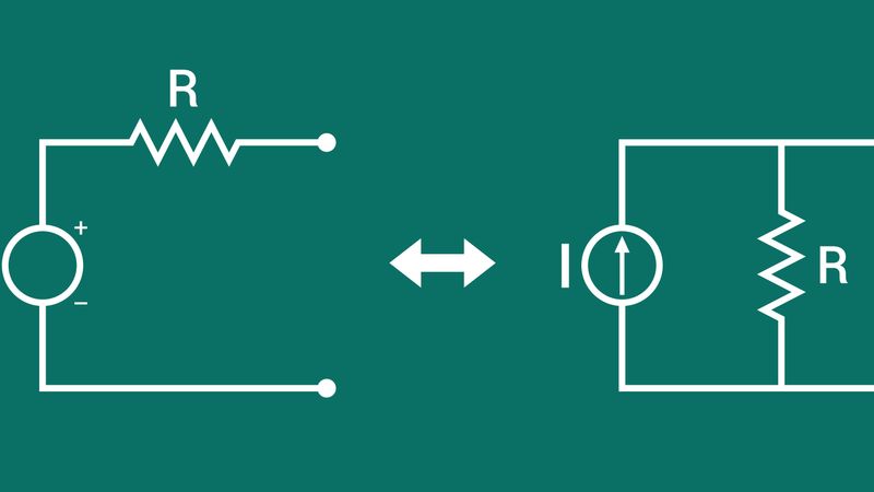
Source transformation is a circuit simplification technique that converts a voltage source in series with a resistor into an equivalent current source in parallel with the same resistor, and vice versa. In other words, any practical voltage source (with some internal resistance) can be “transformed” into an equivalent current source (with the same resistance), without changing how the circuit behaves from the outside.
This process is fundamentally based on Thévenin’s and Norton’s theorems. It exploits the fact that a Thévenin form (voltage source VTh in series with resistance RTh) and a Norton form (current source IN in parallel with resistance RN are mathematically equivalent representations of the same linear two-terminal network. The key idea is that as long as the open-circuit voltage and short-circuit current are preserved, the source can be represented in either form, simplifying circuit analysis.
Suggested Reading: Open Circuit vs Short Circuit: Core Differences between Open and Closed Circuit
Ohm’s Law - The Foundation of Source Transformation
Ohm’s Law is the guiding principle for transformation. So, the equivalent current source value is given by:
In =Vth x Rth ;
And the equivalent voltage source value is:
Vth =In x Rn ;
with the resistance remaining the same, i.e.,
Rn =Rth
For example, a 10 V voltage source in series with a 5 Ω resistor can be transformed into a 2 A current source in parallel with a 5 Ω resistor, yielding an equivalent external behavior.
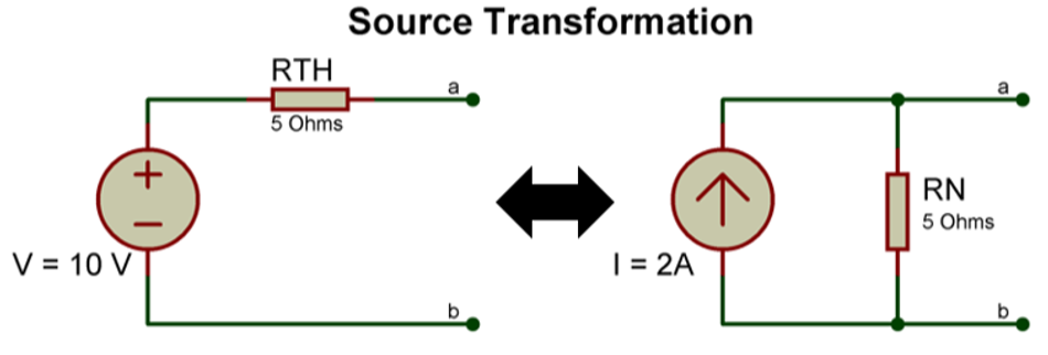
In both configurations, any load connected to the terminals will draw the same current and see the same voltage, affirming that the two sources are equivalent in their effect on the rest of the circuit. Source transformations are extremely useful for circuit simplification, allowing engineers to swap between forms for easier analysis, such as simplifying series/parallel combinations or mesh/nodal analysis.
Why is Source Transformation Possible?
Source transformation works because of the linear V–I relationship at the terminals: any linear two-terminal source and resistor network has a unique IV characteristic that can be maintained in either form.
Thévenin’s theorem guarantees that a linear circuit can be reduced to a single voltage source and series resistance.
Norton’s theorem guarantees an equivalent current source and parallel resistance.
Source transformation is essentially a direct interchange between the Thévenin and Norton equivalents. For linear components, the external port behavior (voltage-current relationship seen by the load) remains unchanged by the transformation.
Thévenin–Norton Equivalence Theory
To understand source transformation deeply, it’s important to recall the Thévenin and Norton equivalence theory behind it:
Thévenin’s Theorem
Any linear circuit with sources and resistances can be reduced to a single voltage source VTh in series with a resistance RTh, as seen from two output terminals. The voltage VTh is the open-circuit voltage at the terminals (no load attached), and RTh is the equivalent resistance of the circuit as seen from the terminals with all independent sources turned off (voltage sources shorted, current sources opened). This Thévenin equivalent will produce the same output voltage and current for any given load as the original circuit.
Norton’s Theorem
Similarly, any linear circuit can be reduced to a single current source IN in parallel with a resistance RN, producing the same behavior at the terminals. The Norton current IN is the short-circuit current flowing between the output terminals (when they are shorted together), and RN (the Norton resistance) is again the equivalent resistance seen from the terminals (which for linear circuits is the same value as RTh under the same conditions).
Importantly, Thévenin and Norton forms are interchangeable. This means a Thévenin-equivalent circuit and a Norton-equivalent circuit are two representations of the same underlying behavior. Source transformation is the practical method of converting a given source into its Thévenin or Norton counterpart.
From an analytical perspective, Thévenin–Norton equivalence is very powerful, implying that any complex linear circuit, no matter how many sources and resistors it has, can be condensed into one source and one resistor to analyze its interaction with the rest of a system.
Recommended Reading: Types of Circuits: A Comprehensive Guide for Engineering Professionals
How to Perform a Source Transformation (Step-by-Step)
Converting a source from one form to the other is straightforward. Below is a general step-by-step procedure:
Identify a Source-Resistor Pair - Locate a portion of the circuit that consists of a voltage source in series with a resistor, or a current source in parallel with a resistor. It is important to note that the source and resistor must be directly in series or parallel with each other and not with other elements in between. (For example, a voltage source with a series resistor that is directly connected to the rest of the circuit at two nodes qualifies.
Calculate the Equivalent Value - Use Ohm’s law to find the transformed source value. If you have a voltage source Vs in series with R, compute Is = Vs / Rs – this will be the value of the equivalent current source. If you have a current source Is in parallel with R, compute Vs = Is R to find the equivalent voltage source value. The resistance value remains the same in both forms (it becomes the parallel resistor for a current source, or the series resistor for a voltage source).
Maintain Polarity and Direction - When substituting the new source in, be careful to keep the correct orientation. The positive terminal of the voltage source corresponds to the arrow direction of the current source. In practice, if a voltage source Vs with a given polarity is converted to a current source, the current arrow should leave the positive terminal of the original voltage source (meaning the current source drives current in the same direction that the voltage source would drive a positive current). This ensures the transformed source delivers power with the same orientation into the circuit.
Replace the Circuit Portion with the Equivalent Source - Remove the original source and its series/parallel resistor, and replace them with the computed equivalent source and resistor. Make sure the resistor is now in parallel with the current source (if you converted from a voltage source) or in series with the voltage source (if you converted from a current source). The connection nodes to the rest of the circuit should remain the same.
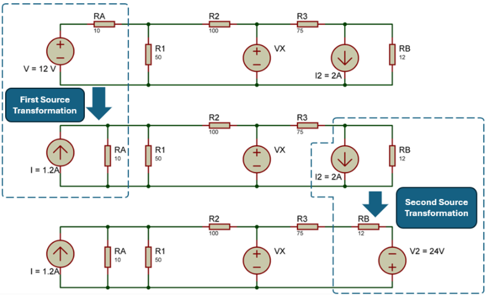
Simplify and Repeat - After the transformation, you may have simplified that section of the circuit (for instance, you might now have two current sources in parallel that you can combine, or two resistors in series, etc.). Continue analyzing or simplifying the circuit. You can perform multiple source transformations in succession if needed, transforming different parts of the circuit step by step until it’s easy to solve.
Applying Source Transformations to Dependent Sources
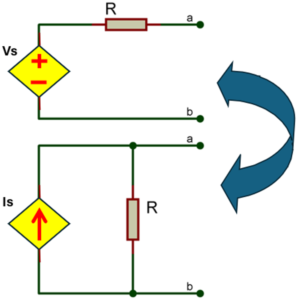
While source transformation is generally applied to independent sources, it can also be applied to dependent sources under certain conditions. Circuits that contain dependent sources require careful handling because a dependent source’s value is tied to some other part of the circuit. A straightforward source transformation may break or change the dependency, leading to an incorrect circuit representation.
If the controlling variable of the dependent source is internal to the source-resistor module being transformed (for example, a voltage-controlled voltage source in series with a resistor, where the controlling voltage is across that resistor or source itself), then an equivalent dependent current source can be derived mathematically.
In such a case, from the perspective of the external terminals, you might be able to transform it “freely” without affecting the rest of the circuit, because the dependency travels along with the transformation.
However, this situation is somewhat unusual. More commonly, the dependent source is controlled by a variable elsewhere in the circuit (external to the source and resistor being considered). In those cases, performing a direct transformation can sever the connection between the control variable and the dependent source or otherwise misrepresent it.
As a rule of thumb, most textbooks advise not to use source transformation on dependent sources unless you’re sure the dependency is preserved. For example, consider a voltage-dependent voltage source in series with a resistor. If its controlling voltage is somewhere else in the circuit, turning it into a current source would require that current to somehow remain a function of that distant voltage – the transformed model might be more confusing than helpful, or even invalid if the dependency path changes.
Unless the dependency is directly on the same source you’re transforming (essentially making it an independent source for that moment), a source transformation isn’t straightforward.
Handling Circuits with Dependent Sources
One approach to handle dependent source circuits is to use the Thévenin/Norton theorem in its general form. Thévenin’s theorem can be applied to circuits with dependent sources by injecting a test source to find RTh, for instance. In analysis, you would keep the dependent source in place and calculate the open-circuit voltage and short-circuit current at the terminals using circuit analysis techniques (superposition, node-voltage method, etc.).
This yields a Thévenin or Norton equivalent that may itself contain a dependent source, or at least accounts for it. But you typically would not switch forms back and forth casually with dependent sources.
Simply put, source transformation is mostly used in circuits with independent sources (linear circuits with fixed sources). It requires extra caution if dependent sources are present, eventually forcing other analysis methods to include the effect of dependent sources.
AC Source Transformations (Impedances and Phasors)
The concept of source transformation naturally extends to AC circuit analysis using phasors and impedances.
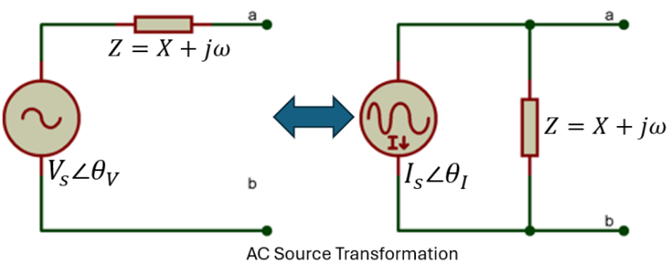
AC source transformation follows the same principle: an AC voltage source in series with an impedance Z can be converted to an AC source in parallel with the same impedance Z, and vice versa. The key differences are just that voltage and current are expressed as phasors, and resistances generalize to impedances.
Suggested Reading: Calculate Impedance in AC Circuits: A Comprehensive Guide for Engineers
To perform a source transformation in AC circuits:
Identify a voltage source VS∠𝚹v in series with an impedance Z = R + jX or a current source IS∠𝚹i in parallel with Z.
Use the same formulas - Is = Vs / Z or Vs = Is Z. The impedance Z remains the same in both forms.
Maintain phase relationships - The polarity of the voltage source and reference direction of the current source must correspond. If the original AC voltage source had a phase angle 𝚹, the resulting current source will have phase $\theta$ as well (plus any phase shift from dividing by a complex Z.
Replace and analyze in the phasor domain just as you would in DC, treating Z like a “resistance”.
In AC circuits, source transformations are particularly handy for simplifying circuits before using nodal or mesh analysis. For instance, you might convert all sources to phasor current sources and combine them if they are in parallel (superposition in current form), or convert to voltage sources in series if that makes loops easier to sum via KVL. The technique also works when dependent sources and impedances are present, with the same caveats discussed earlier (linearity and careful attention to dependencies).
It’s worth noting that source transformations in AC have the same limitations as in DC: the circuit must be linear and bilateral. Also, you cannot transform a source if the impedance is not clearly in series/parallel with it as required.
Common Mistakes and Pitfalls in Source Transformation
While source transformation is a straightforward tool, there are several common mistakes and edge cases to be mindful of:
Not meeting the conditions for transformation - You can only perform a source transformation when a voltage source is in series with a single resistor or a current source is in parallel with a single resistor. A direct transformation isn't valid if additional elements are present or the configuration isn't a pure source-resistor pair; you must first isolate the proper source-resistor pair through circuit reconfiguration.
Reversing polarity or direction - A frequent error is reversing the polarity or direction of the source during transformation. The direction of the equivalent current source and the polarity of the equivalent voltage source must correspond to deliver power identically. To ensure correctness, mark the positive terminal of the voltage source and verify that the current source arrow points from positive to negative through the resistor, or vice versa for current-to-voltage conversion.
Forgetting to transform the resistor or misplacing it - It's crucial to transform the resistor along with the source and ensure it's placed correctly. The resistor's value remains unchanged, but its configuration shifts from series to parallel (or vice versa) with the new source. Omitting or misplacing the resistor will drastically alter the circuit's behavior, as the resistor is an integral part of the source model.
Applying source transformation in non-linear or time-varying contexts - Source transformation is strictly for linear and time-invariant circuits. This technique doesn't apply to circuits containing non-linear elements (like diodes or transistors in active regions) or time-varying components in the time domain. For such circuits, alternative analysis methods or transformations to other domains (e.g., s-domain or phasors) are necessary.
Expecting internal quantities to remain the same - While external circuit behavior remains identical after a source transformation, the internal distribution of voltage, current, and power between the source and its resistor may differ. This is normal, as only the external port behavior is guaranteed to be the same. When calculating power, be consistent and remember that the total power delivered to the rest of the circuit remains unchanged.
Ideal source edge cases - Be cautious when dealing with ideal sources (zero or infinite internal resistance), as they generally cannot be directly transformed into a finite equivalent. Attempting to transform them often results in nonsensical values. Source transformation is typically applied to practical sources with finite internal resistance, or you may need to incorporate an external resistor from the network to create a transformable combination.
Losing sight of the big picture - Use source transformations strategically as a means to simplify the circuit, not as an end in itself. Avoid aimless transformations that don't reduce complexity. Always consider your ultimate goal—such as combining sources or simplifying a circuit for a specific analysis—to ensure each transformation contributes to a more straightforward solution.
Conclusion
Even with the rise of advanced electrical engineering domains like digital twin modeling and transient analysis, source transformation remains a vital tool. Digital twins, which are software models emulating real electrical systems, frequently leverage Thévenin or Norton equivalents to simplify complex hardware like power supply units or battery packs. These simplified models, derived using source transformation principles, allow for real-time and efficient computation by abstracting detailed sub-networks into equivalent sources and impedances. This enables accurate simulation of subsystem behavior under various conditions without the overhead of full, detailed circuits.
Furthermore, source transformation is crucial in transient analysis for simplifying initial conditions and equivalent circuits. For instance, it allows engineers to determine the time constant of RC or RL circuits by reducing the surrounding network to a Thévenin equivalent. This approach streamlines the differential equations, making it easier to analyze dynamic behavior. The ability of source transformations to preserve steady-state characteristics also extends their utility to complex scenarios like power system fault analysis and high-speed digital electronics, where simplified models are essential for predicting interactions and ensuring signal integrity.
Suggested Reading: Digital Twins bridge the gap between product development and product operations
FAQs
What is source transformation in circuit analysis?
Source transformation is a method of simplifying circuits by converting between an equivalent voltage source and current source. Specifically, a voltage source in series with a resistor can be converted into a current source in parallel with the resistance, and vice versa. This does not change the external behavior of the circuit – any load connected will see the same voltage-current characteristics. It’s a direct application of Thévenin’s and Norton’s theorems to swap the form of sources while preserving circuit equivalence.
What are the advantages of using source transformation?
Source transformation makes circuit analysis more flexible and often easier. Key advantages include:
Simplification: It can reduce a complex circuit into simpler series/parallel groups. For instance, multiple sources can be combined after transforming them to the same type (all voltage or all current). This often means fewer equations to solve.
Intuitive problem-solving: It allows you to choose the form (voltage or current) that best fits the analysis at hand (e.g., using a Norton form for nodal analysis or Thévenin form for mesh analysis or when connecting to a load).
Clarity in design: Engineers use source equivalents to understand how a circuit behaves “as seen” by a load or another circuit. For example, modeling a sensor or a power supply as a Thévenin equivalent (via source transformation) makes it easier to predict its interaction with varying loads.
Computational efficiency: In large circuits or repeated calculations (like iterative simulations), replacing parts of the circuit with their source equivalents can greatly speed up computations by reducing circuit complexity without sacrificing accuracy. This is why source transformations are popular in simulation and digital twins modeling, as well as hand analysis.
How is source transformation related to Thévenin’s and Norton’s theorems?
They are closely related – essentially two sides of the same coin. Thévenin’s theorem provides a way to reduce a network to a single voltage source and series resistance. Norton’s theorem does the same with a current source and parallel resistance. In practice, if you’ve found a Thévenin equivalent, you can get the Norton equivalent directly (and vice versa) – the resistor stays the same. Source transformation can also be used during the process of finding a Thévenin/Norton equivalent: one method to find a Norton equivalent is to first find the Thévenin, then transform it. All three concepts are applicable only in linear circuits. In summary, source transformation is basically applying Thévenin/Norton ideas locally to swap a source’s representation.
Can source transformations be applied to AC circuits?
Yes. Source transformations work in AC circuit analysis as long as you use impedances (the complex generalization of resistance) and phasor representations of sources. This is valid because AC circuit equations are linear (for a fixed frequency), so the same linear principles apply. It’s commonly used in AC network simplification and power engineering.
Can you perform source transformation with dependent sources?
It’s not generally recommended to directly transform dependent sources unless the dependency is internal to the source-resistor module being transformed. The reason is that a dependent source’s value is tied to some other circuit variable, and converting the source could break that relationship or remove the controlling variable from where it’s needed. For example, a current-controlled voltage source in series with a resistor shouldn’t be blindly turned into a current source, because the current that controls it might flow differently in the new form. In circuits with dependent sources, it’s safer to use formal Thévenin/Norton derivation techniques (like inserting a test source to find $R_{Th}$) while keeping the dependent source intact in the equations. If the dependent source is controlled by a variable within the subcircuit you’re transforming, mathematically it can be converted (the dependency will carry over), but such cases are specific. In summary, treat dependent sources with care: linearity allows Thevenin/Norton equivalents to exist with dependents, but routine source transformation shortcuts are usually not applicable.
References
W. McAllister, "Source transformation," Spinning Numbers – Electronics Tutorials. [Online]. Available: https://spinningnumbers.org/a/source-transformation.html.
"Source transformation," Wikipedia, The Free Encyclopedia. [Online]. Available: https://en.wikipedia.org/wiki/Source_transformation.
"Source Transformation with Solved Examples," Tutorials Point. [Online]. Available: https://www.tutorialspoint.com/source-transformation-with-solved-examples.
"Source Transformation," All About Circuits. [Online]. Available: https://www.allaboutcircuits.com/technical-articles/source-transformation/.
"Circuits: Source Transformation Formula," Dadao Energy Blog. [Online]. Available: https://dadaoenergy.com/blog/circuits-source-transformation-formula/.
in this article
1. Key Takeaways2. What is Source Transformation?3. Thévenin–Norton Equivalence Theory4. How to Perform a Source Transformation (Step-by-Step)5. Applying Source Transformations to Dependent Sources6. AC Source Transformations (Impedances and Phasors)7. Common Mistakes and Pitfalls in Source Transformation8. Conclusion9. FAQs10. References