Difference Amplifier: Theory, Design, and Applications for Engineers

Key Takeaways

1. Core Functionality:  A differential amplifier amplifies only the voltage difference between two inputs while rejecting any common-mode noise; the op-amp differential amplifier (also called a difference amplifier) is its most common board-level form. This makes them essential for extracting clean signals in noisy environments, like sensor readings with varying grounds or long cable runs.

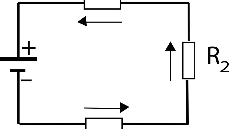
2. Fundamental Design Resistor Network: The typical differential op-amp configuration uses a four-resistor network around the op-amp. The accuracy of the amplifier’s output depends critically on the precise matching of these resistors; the gain directly correlates to the ratio of the feedback to input resistors. When matched correctly, the amplifier provides stable and distortion-minimized performance.

3. High Common-Mode Rejection Ratio (CMRR): A difference amplifier’s (or differential amplifier's)  strength lies in its ability to suppress noise effectively, but this depends heavily on resistor matching. Well-matched resistors yield a high CMRR, enabling the rejection of unwanted signals common to both inputs.

4. Distinguishing from Instrumentation Amplifiers: While both op amp differential amplifiers and instrumentation amplifiers handle differential inputs, the latter include input buffering and adjustable gain, which makes them better for low-level, high-impedance sources. The guide helps engineers decide which type suits their specific application needs.

5. Design Tips & Practical Implementation: The article doesn’t just stop at theory; it provides practical advice on component selection, matching resistor tolerances, and managing impedance to ensure stable operation. These detailed insights help transform a precision signal measurement from a complex challenge into a reliable, repeatable design process.

6. From Transistor Pair to Precision Circuit: Every op amp is built around a transistor differential pair, the long-tailed pair. Understanding this stage explains where CMRR, input offset voltage, and common-mode limits come from, and why the four-resistor difference amplifier is the practical choice for board-level measurement.

Introduction

In many analog circuit applications, engineers face the challenge of extracting tiny differential signals from a noisy environment. Whether it’s measuring a microvolt-level voltage drop across a shunt resistor, reading sensor data with varying ground potentials, or dealing with interference in long cable runs, unwanted common-mode voltage can distort readings and degrade performance. Traditional amplifier circuits often struggle here, as mismatched components or low CMRR allow noise to leak into the output, making accurate measurement nearly impossible.

A small voltage amplification circuit

The differential amplifier solves this problem by amplifying only the voltage difference between two input terminals while rejecting the noise both inputs share. The term covers a family of circuits, from the transistor differential pair inside virtually every op amp to fully differential ICs, but its most common board-level form is the difference amplifier: an operational amplifier with a carefully matched four-resistor network, also called an op amp differential amplifier or differential op amp. This configuration provides engineers with a high-performance subtractor featuring predictable differential gain, stable operation, and compatibility with both discrete op-amp circuits and integrated circuits. 

In this guide, you’ll learn what is a differential amplifier, the transistor-level differential pair, circuit design considerations, and practical implementation tips, plus how to choose between a difference amplifier and an instrumentation amplifier for your specific electrical engineering needs. From improving common mode rejection ratio to optimizing impedance and feedback resistor values, we’ll cover the essentials that turn precision signal measurement from a headache into a reliable design advantage.

What Is a Differential Amplifier?

A differential amplifier is a broad category of electronic circuit that amplifies the voltage difference between two input signals while rejecting any voltage common to both,  known as common-mode noise. 

Differential Amplifier Circuit Diagram

The term covers a wide range of circuits: the transistor-level differential pair found inside virtually every op-amp, fully differential ICs, instrumentation amplifiers, and the board-level difference amplifier built from a single op-amp and four resistors.

Fundamentals of Differential Amplification

At its core, a difference amplifier is an operational amplifier (op-amp) circuit designed to output a signal proportional to the voltage difference between two input signals, while rejecting any common-mode voltage they share. This precise operation relies on a network of carefully matched resistors that set the amplifier’s gain and maintain balanced signal paths. When both inputs carry the same unwanted noise or interference, the amplifier’s high common-mode rejection ratio (CMRR) effectively cancels it out, leaving only the clean differential signal at the output.

Unlike simpler amplifiers that work with a single input, difference amplifiers handle differential inputs, typically implemented with a four-resistor configuration around the op-amp to form a stable subtractor circuit. The accuracy of the output voltage depends not just on the resistor ratio that sets the gain, but on how precisely that ratio matches between both resistor pairs (R2/R1 = R4/R3); any mismatch between the two ratios directly degrades CMRR.  When these are perfectly matched, the circuit amplifies the difference without distorting the original signal. This design principle is foundational for instrumentation amplifiers, which add buffer stages for high input impedance and adjustable gain, making them ideal for low-level sensor signals.

In the context of building better PCBs, understanding these fundamentals is crucial [4]. Proper PCB layout (precision placement of components, careful routing of resistor networks, and symmetrical trace lengths) helps maintain the balance and noise rejection capabilities of difference amplifiers. This attention to detail ensures that the amplifier performs optimally on the board, resulting in more accurate and reliable analog signal processing.

This image shows a close-up of a printed circuit board (PCB) with an integrated circuit (IC) die connected via fine gold bonding wires.

Recommended Reading: VSS vs VDD: Understanding Power Rails in Electronic Circuit Design

Common-mode Rejection Ratio (CMRR)

One of the most important performance metrics in any difference amplifier or instrumentation amplifier is its common-mode rejection ratio (CMRR). CMRR measures how effectively the amplifier circuit rejects unwanted common-mode voltage (the identical signal present on both input terminals) while amplifying only the desired voltage difference. In electrical engineering terms, it’s the ratio of differential gain to common-mode gain, usually expressed in decibels. A high CMRR ensures that interference from power lines, ground loops, or electromagnetic noise does not appear at the output voltage.

Achieving a high CMRR in op-amp circuits depends heavily on precision resistor matching. Even a small mismatch in feedback resistor or input resistor values can introduce an imbalance, allowing a portion of the noise to pass through. 

For example, using 1% tolerance resistors typically limits CMRR to around 34 dB, while 0.1% tolerance resistors improve this to roughly 66 dB. Achieving CMRR beyond 100 dB generally requires laser-trimmed, integrated difference-amplifier ICs with internally matched resistors, rather than discrete components. Proper circuit design also accounts for temperature effects, as resistor drift can degrade matching over time. In high-performance applications, such as sensor signal conditioning, medical instrumentation, and industrial process control, a strong CMRR is critical for maintaining accuracy and reliability in the presence of large common-mode voltages.

Terminology: Difference vs. Differential Amplifiers

In electrical engineering, the terms difference amplifier and differential amplifier are often used interchangeably, but they describe related, yet distinct, amplifier circuits. A difference amplifier is a specific op-amp circuit configuration, typically built with a four-resistor network, that produces an output voltage proportional to the voltage difference between two input signals while rejecting common-mode voltage. It’s essentially a precision subtractor and serves as the core building block for many instrumentation amplifiers [7].

In contrast, a differential amplifier is a broader term for any amplifier designed to amplify the difference between two input signals. It can be built using transistors, op-amps, or integrated circuits [3]. This category includes the transistor-level differential pair (the long-tailed pair covered later in this guide) and fully differential amplifiers that provide differential outputs instead of a single-ended one. These are common in high-speed analog circuits, ADC drivers, and balanced line transmission, where matched impedance and symmetrical signal paths are critical. While both topologies rely on the same amplification principle, the difference amplifier excels in simple, cost-effective circuit designs requiring stable gain and good CMRR, whereas fully differential amplifiers are favored in systems needing greater noise immunity, symmetrical feedback paths, and the wider dynamic range of differential outputs.

Recommended Reading: Calculate Impedance in AC Circuits: A Comprehensive Guide for Engineers

Common-Mode Range

The common-mode range of a difference amplifier defines the span of common-mode voltages at the input terminals that the amplifier circuit can handle without distortion or loss of accuracy. In many op-amp circuits, this range is limited to within the power supply rails. However, certain precision integrated circuits, such as the Texas Instruments INA149, use carefully designed resistor networks to attenuate the input voltage, allowing them to operate with common-mode levels far beyond the supply limits. This capability makes them ideal for high-side current sensing, battery stack monitoring, and industrial measurements where large offsets are unavoidable.

In practical circuit design, understanding the common-mode range is critical to ensuring that both differential gain and CMRR remain stable across the full range of operating conditions. For example, a difference amplifier with ±275 V common-mode range can monitor signals in high-voltage systems without isolation, whereas a typical instrumentation amplifier may be restricted to ±15 V. Selecting the right device means balancing your required input voltage range, impedance needs, and feedback resistor configuration to achieve reliable amplification under real-world conditions.

Recommended Reading: Types of Circuits: A Comprehensive Guide for Engineering Professionals

Input Impedance and the Need for Buffers

In a standard four-resistor difference amplifier configuration, the input impedance seen at each input terminal is not only moderate but also unequal. The non-inverting input typically sees a single resistor path, while the inverting side must drive a feedback resistor network to ground. This asymmetry can load the signal source unevenly, especially in amplifier circuits connected to high-impedance sensors. If the voltage source cannot supply enough current, the measured output voltage may suffer accuracy loss and degraded CMRR.

To overcome this, designers often add op-amp buffer stages, unity-gain non-inverting amplifiers, ahead of the difference amplifier [5]. These buffers present high input impedance to the source and isolate it from the feedback resistor network, ensuring that the differential gain remains accurate. This buffered approach is the basis of the instrumentation amplifier, which combines two input buffers with a subtractor stage to deliver exceptional common-mode rejection ratio and flexible gain settings. In high-precision circuit design, especially for differential signals from sensors like strain gauges or thermocouples, using buffers is essential to preserve signal integrity, minimize loading, and maintain predictable amplification across the operating range.

Instrumentation Amplifier Basics

An instrumentation amplifier is built using two non-inverting buffer amplifiers followed by a differential subtractor stage. The buffer amplifiers provide high input impedance, which prevents loading of the input signals, and their gain is controlled by external resistors. The gain of each buffer stage is given by the formula: Gain_buffer = 1 + (2 × R2) / R1, where R1 and R2 are the external resistors.

Instrumentation Amplifier Circuit

The subtractor stage amplifies the difference between the two buffered signals, rejecting any common-mode voltage present on both inputs. This arrangement allows the overall gain of the instrumentation amplifier to be easily adjusted by changing just one resistor that connects the two buffer stages. Well-designed three-op-amp instrumentation amplifiers can achieve common-mode rejection ratios (CMRR) above 100 dB, enabling them to amplify small differential signals accurately even in noisy environments [1].

Instrumentation amplifiers are commonly available as integrated circuits with built-in precision resistor networks for stable and accurate gain. For example, the Texas Instruments INA828 offers extremely high input impedance, around 100 gigaohms (GΩ), making it ideal for sensitive sensor measurements [8]. However, its common-mode voltage range is limited to within about 2 V of its supply rails, with dual supplies up to ±18 V. In contrast, difference amplifiers such as the INA149 sacrifice input impedance; dropping to 800 kΩ differential / 200 kΩ common-mode to handle very large common-mode voltages, which is useful in industrial applications where signals may be referenced to high voltages. These trade-offs highlight the importance of choosing the right amplifier type based on the application's input impedance and common-mode voltage requirements.

The Differential Pair: The Transistor Circuit Virtually Inside Every Op Amp

At the transistor level, a differential amplifier starts with two matched transistors, either BJTs or FETs, joined at their emitters or sources. This circuit is called a differential pair, or long-tailed pair, and it forms the input stage of virtually every operational amplifier, as well as of comparators and high-speed interface ICs.

The joined node is biased by a tail current source: a resistor in the simplest designs, an active current source built around a current mirror in integrated circuits. Because the tail current is fixed, a signal that appears in phase on both inputs cannot change the total current through the pair, so it produces almost no output. The higher the output impedance of the tail current source, the lower the common mode gain and the better the CMRR [7].

A differential input signal, by contrast, steers the tail current from one transistor to the other. Each half of the pair then behaves like one of the classic single-ended amplifiers, a common emitter amplifier for BJTs or a common source stage for MOSFETs. You can take the output from one collector or drain as a single-ended output, or from both as a differential output. In integrated designs, a current mirror often replaces the load resistors, converting the pair's differential current into a single-ended output while leaving common-mode components behind. The pair's transfer function is linear only for small differential inputs, which is why practical amplifiers wrap it in negative feedback [3].

Matching matters as much here as in the four-resistor circuit. Any mismatch between the two transistors unbalances the pair and shows up as input offset voltage and degraded common-mode rejection, which is why op amp input stages use tightly matched monolithic pairs rather than separate discrete transistors.

So when should you build a discrete long-tailed pair instead of using an op amp? Rarely, for measurement work. An op amp already contains a differential pair wrapped in additional gain stages and negative feedback, giving you stable, resistor-set gain without transistor-level design effort. Discrete BJT or MOSFET pairs still earn their place inside custom ICs, in radio-frequency front ends beyond an op amp's bandwidth, and in the classroom, where they explain exactly where an op amp's CMRR, offset, and common-mode limits come from.

Practical Design and Implementation

Building a reliable difference amplifier comes down to balancing a few interlocking trade-offs. Here's what to weigh:

Resistor Selection and CMRR

The differential gain is set simply by the resistor ratio: Gain = R2/R1. For example, R2 = 10 kΩ and R1 = 1 kΩ gives a gain of 10. But resistor tolerance, not just the ratio determines your real-world CMRR. A quick estimate: CMRR ≈ Gain / tolerance (as a decimal), converted to dB via 20 × log₁₀(value). At unity gain, 1% resistors land you around 34 dB; tightening to 0.1% gets you to roughly 54–66 dB (the exact figure depends on how the mismatch is distributed across the network see the CMRR section above for the full explanation). For anything beyond that, matched resistor networks or laser-trimmed integrated difference-amplifier ICs are the practical path.

Noise vs. Impedance Trade-off

Resistor value choice cuts both ways: lower-value resistors reduce thermal noise but load the source harder (worsening the impedance mismatch discussed earlier); higher-value resistors ease that loading but add more noise and limit bandwidth. Some difference amplifier ICs address this with built-in input filtering or feedback-network capacitors to help stabilize the circuit.

Real-world Protection

Since input resistors in integrated difference amplifiers sit directly in the common-mode voltage path, they need to handle more than just the expected signal transient spikes and overvoltage events included. The INA149, for example, includes input protection rated to ±500 V, well beyond its ±275 V operating range, specifically for this reason. This is a good reminder that protection headroom, not just nominal specs, matters in harsh industrial environments.

Real-World Difference Amplifiers Comparison

INA828 and INA152 by Texas Instruments

Example Discrete Difference Amplifier Design

Suppose you need to measure a 5 V shunt voltage across a high-side current-sense resistor in a 48 V system. To scale this voltage for an ADC, you choose a gain of 0.1 (or 1/10) so the output voltage is 0.5 V. A discrete difference amplifier can be built using four resistors:

R1 = 10 kΩ

R2 = 1 kΩ

R3 = 10 kΩ

R4 = 1 kΩ

This resistor combination provides the required gain of 0.1, calculated as:

Gain = R2/R1 (when R1 = R3 and R2 = R4) = 1 kΩ/10 kΩ = 0.1 

(Note: In a classic difference amplifier with matched resistor pairs, gain is often simplified to R2 / R1 when R1 = R3 and R2 = R4.)

However, to maintain a high common-mode rejection ratio (CMRR) and avoid errors caused by the 48 V common-mode voltage, the resistors must have a tight tolerance, ideally 0.1%. If the resistor tolerance is insufficient, the output voltage will include errors from common-mode signals. Alternatively, you can use an integrated difference amplifier with internally matched resistors and pin-strappable gain settings, such as the LT1991, to achieve high CMRR without hand-matching precision resistors [10]. If the sensor or source impedance is high or if additional filtering is required, an instrumentation amplifier such as the INA826 with gain set to 10 is a suitable option.

Difference Amplifier vs Instrumentation Amplifier

Instrumentation amplifiers are often seen as an advanced form of the difference amplifier. The table below compares their main features:

Choosing Between Difference and Instrumentation Amplifiers

Engineers should choose a difference amplifier when the signal is floating or has a large common-mode voltage, when cost and size matter, or when moderate input impedance is acceptable. For example, high-side current sensing in automotive and industrial systems benefits from difference amplifiers because they reduce the high supply voltage while accurately amplifying the small shunt voltage. They are also ideal for ground loop isolation in audio and data acquisition systems.

On the other hand, instrumentation amplifiers are best when the signal source has a high impedance or when very small differential signals (in microvolts) require high gain [1]. Common applications include strain gauges, thermocouples, and biomedical sensors like ECG electrodes. The high input impedance of instrumentation amplifiers prevents loading the sensor, and their adjustable gain lets engineers scale the signal by changing a single external resistor, rather than a full matched resistor network [8].

Closeup view of ECG electrodes attached to patient’s arms

Applications in Modern Electronics

Current Sensing 

Measuring current often involves sensing the voltage drop across a shunt resistor. When the shunt is placed on the high side of a supply line, the voltage signal is combined with a large common-mode voltage from the supply. A difference amplifier amplifies only the small shunt voltage while rejecting the high common-mode voltage. High-side current-sense amplifiers like the INA149 or LT1991 offer wide common-mode ranges and built-in protection. Low-side current sensing also benefits from differential amplifiers when ground drops cause measurement errors.

Ground Loop Isolation and Signal Transmission

When two circuits have different ground potentials, connecting them directly can create noise-inducing ground loops. A difference amplifier solves this by measuring only the voltage difference between the signals, ignoring offsets caused by differing grounds. This method is widely used in instrumentation, audio gear, communication systems, and industrial control.

Battery Monitoring and Cell Balancing

Battery packs in electric vehicles and portable devices consist of many cells in series, creating high common-mode voltages relative to ground. Monitoring each cell requires amplifiers with a high common-mode range. Difference amplifiers integrated into battery-monitor ICs can measure individual cell voltages without isolation. For example, amplifiers with a ±275 V common-mode range can handle roughly 65–75 lithium-ion cells in series (at typical 3.6–4.2 V per cell) on supplies as low as ±2 V. 

Applications of Difference Amplifiers

Sensor Signal Conditioning

Many sensors output small differential voltages. Strain gauges in Wheatstone bridges, RTDs, and thermocouples generate tiny signals with high source impedance. Instrumentation amplifiers are ideal here because of their very high input impedance and adjustable gain [2]. However, difference amplifiers can be used with low-impedance sources like Hall effect current sensors or microphones when common-mode voltage rejection is needed.

Audio and Video Processing

Difference amplifiers extract difference signals from balanced audio or stereo lines, rejecting hum and noise. They are common in audio preamplifiers and balanced line receivers. High-speed video difference amplifiers like the LT1193 offer adjustable gain and bandwidth up to 80 MHz, suitable for composite video applications and differential communication drivers.

Automotive and Industrial Control

Automotive motor controllers, battery management, and sensor interfaces operate in noisy environments with high supply voltages. Difference amplifiers are used to monitor high-side currents, battery cells, and sensors while handling transient voltages and electromagnetic interference. In industrial control, they measure motor currents, process variables, and prevent ground loop issues.

Medical Instrumentation

Systems like ECG and EEG require amplifying microvolt-level signals from body electrodes. Instrumentation amplifiers dominate here due to their high input impedance and excellent CMRR [2]. Difference amplifiers may be used later in the signal chain to remove residual common-mode noise or handle signals with moderate source impedance. The rise of wearable health devices continues to drive demand for precision difference and instrumentation amplifiers.

Man use smart watch for health care technology monitoring

Recommended Reading: PCBA Manufacturing: Revolutionizing Modern Electronics Assembly

Market Trends and Future Outlook

The demand for difference amplifiers and instrumentation amplifiers is growing alongside the expansion of precision sensing and control technologies. Market size was valued at USD 2.5 Billion in 2024 and is poised to grow from USD 2.8 Billion in 2025 to USD 4.2 Billion by 2033, growing at a CAGR of 5.2% during the forecast period 2026-2033 [6].

Key growth drivers include the increasing need for accurate current measurement in electric vehicles and renewable energy systems, the rise of IoT networks, and ongoing miniaturization in consumer electronics.

Instrumentation amplifiers track the same demand for precision sensing and continue to be essential components in medical devices, industrial sensors, and data acquisition systems.

These trends highlight a rising demand for amplifier circuits that offer high precision, low noise, and a strong common-mode rejection ratio (CMRR). As autonomous vehicles, renewable energy installations, and smart factories become more widespread, engineers will increasingly depend on difference and instrumentation amplifiers to interface with sensors, accurately monitor current, and enable safe, reliable control in complex systems.

Conclusion

Difference amplifiers are essential building blocks in electronics that subtract and amplify two input signals while rejecting common-mode noise. Their basic design uses four resistors to produce an output proportional to the voltage difference, with gain set by resistor ratios. Achieving a high common-mode rejection ratio (CMRR) requires precise resistor matching and careful circuit layout or the use of integrated devices. In contrast, instrumentation amplifiers add buffer stages and adjustable gain, offering very high input impedance and more flexibility, though usually with a smaller common-mode voltage range.

When designing measurement or control systems, engineers must balance trade-offs between input impedance, common-mode range, gain, cost, and noise performance. Integrated difference amplifiers like the INA149 or configurable devices such as the LT1991 simplify high-side voltage measurements without isolation, while instrumentation amplifiers like the INA828 are ideal for amplifying small sensor signals. Market trends show increasing demand for both amplifier types as fields like electric vehicles, industrial automation, and medical instrumentation require ever more precise and interconnected sensing solutions.

Frequently Asked Questions (FAQ)

What is the key difference between a difference amplifier and an instrumentation amplifier? 

A difference amplifier uses a single op-amp with four resistors to amplify the difference between two inputs, while an instrumentation amplifier adds two input buffers for much higher input impedance and single-resistor gain adjustment. 

How does a difference amplifier achieve common-mode rejection? 

The resistor network forms two voltage dividers that attenuate common-mode voltage by the same ratio at each input, so the op-amp, which only amplifies the difference between its two inputs sees no common-mode difference to amplify. This cancellation depends on precise resistor matching; otherwise, some common-mode voltage leaks through as an error  

Why are resistor tolerances critical in difference amplifiers?

CMRR depends directly on how closely the resistor pairs match; 1% resistors typically limit CMRR to around 34 dB, 0.1% resistors improve this to roughly 66 dB, and laser-trimmed integrated networks can push CMRR beyond 100 dB.  

Can difference amplifiers handle voltages beyond their supply rails?

Yes, the resistor network attenuates the input signal, letting devices like the INA149 handle ±275 V common-mode voltages on just ±2 V to ±18 V supplies. 

When should I use a difference amplifier instead of an instrumentation amplifier?

Choose a difference amplifier for high common-mode voltage, low source impedance, or cost-sensitive designs; choose an instrumentation amplifier for high-impedance sources or small differential signals needing flexible gain. 

What are common applications of difference amplifiers? 

Current sensing, battery monitoring, ground loop isolation, audio/video signal conditioning, and industrial or automotive sensor interfaces are the most common uses. 

Is a differential amplifier the same as a difference amplifier? 

No, a differential amplifier is the broader category (including transistor pairs and fully differential ICs), while a difference amplifier is the specific single-op-amp, four-resistor circuit within that category [7]. 

What is a long-tailed pair? 

A long-tailed pair is two matched transistors sharing a common tail current source, forming the input stage of nearly every op-amp, it rejects common-mode signals while amplifying differential ones [7]. 

How do difference amplifiers relate to fully differential amplifiers?

Fully differential amplifiers have both differential inputs and outputs, offering better noise immunity and signal swing than a standard single-ended-output difference amplifier. 

References

[1] E. Sadiq, "Design of a High Precision Instrumentation Amplifier in 45 nm CMOS Technology," Department of Electrical and Electronic Engineering, Bangladesh University of Engineering and Technology, Final Project Report, 2024. [Online]. Available: https://www.researchgate.net/publication/381561813_Design_of_a_High_Precision_Instrumentation_Amplifier_in_45_nm_CMOS_Technology

[2] F. Moulahcene, N. Bouguechal, and Y. Belhadji, "A Low Power Low Noise Chopper-Stabilized Two-stage Operational Amplifier for Portable Bio-potential Acquisition Systems Using 90 nm Technology," International Journal of Hybrid Information Technology, vol. 7, no. 6, pp. 25–42, Nov. 2014, doi: 10.14257/ijhit.2014.7.6.03

[3] F. Khateb and T. Kulej, "Design and Implementation of a 0.3-V Differential Difference Amplifier," IEEE Transactions on Circuits and Systems I: Regular Papers, vol. 66, no. 2, pp. 513–523, Sep. 2018, doi: 10.1109/TCSI.2018.2866179

[4] A. Abiola, "Building Better PCBs: Key Design Strategies and Modern Manufacturing Tips," NextPCB Blog, Aug. 11, 2025. [Online]. Available: https://www.nextpcb.com/blog/building-better-pcbs-key-design-strategies-and-modern-manufacturing-tips

[5] J. Hertz, "Why JFETs are Key in Low-Noise Sensor Amplification," Wevolver, Jun. 11, 2025. [Online]. Available: https://www.wevolver.com/article/why-jfets-are-key-in-low-noise-sensor-amplification

[6] WiseGuyReports, "Differential Amplifier Market Insights | Size & Outlook 2035," 2025. [Online]. Available: https://www.wiseguyreports.com/reports/differential-amplifier-market

[7] Analog Devices, "Chapter 12: Differential Amplifiers," ADI University Program Electronics Text. [Online]. Available: https://wiki.analog.com/university/courses/electronics/text/chapter-12

[8] Texas Instruments, "INA828 Precision Instrumentation Amplifier," datasheet SBOS562. [Online]. Available: https://www.ti.com/lit/ds/symlink/ina828.pdf

[9] Texas Instruments, "INA152 Single-Supply Difference Amplifier," datasheet SBOS184. [Online]. Available: https://www.ti.com/lit/ds/symlink/ina152.pdf

[10] Analog Devices, "LT1991 Precision, 100 µA Gain Selectable Amplifier," product page. [Online]. Available: https://www.analog.com/en/products/lt1991.html