Controlled Impedance PCB Design: A Comprehensive Guide

Key Takeaways

• Controlled impedance helps preserve signal integrity by limiting reflections caused by impedance discontinuities along a PCB signal path.

• The PCB stackup sets the foundation. Trace width, copper thickness, dielectric thickness, dielectric constant (Dk), and reference-plane geometry determine characteristic impedance.

• Common targets include 50 Ω single-ended and 100 Ω differential impedance, but the required values depend on the interface and system design.

• Impedance tolerances must be agreed upon with the PCB manufacturer. ±10% is a common specification, but acceptable tolerances depend on the application, fabrication capability, and design requirements.

• Routing affects electrical performance. Continuous reference planes, well-designed vias and layer transitions, and appropriate trace spacing help control reflections and crosstalk.

• Test coupons and time-domain reflectometry (TDR) help verify fabrication results. A passing coupon provides evidence of process compliance but does not prove that every signal path on the finished PCB meets its impedance requirement.

Introduction

Controlled impedance is the design and fabrication of PCB signal traces to achieve a specified characteristic impedance within an agreed tolerance. It is important when fast signal transitions make transmission-line effects significant, including in high-speed digital, radio-frequency (RF), and telecommunications circuits.

Changes in trace geometry, dielectric properties, or reference-plane continuity can create impedance discontinuities. These discontinuities may cause signal reflections, ringing, overshoot, and timing errors. Achieving the target impedance therefore requires coordination between PCB layout, material selection, stackup design, and fabrication.

This guide explains the main controlled-impedance structures, the factors that determine impedance, how to design and specify a PCB for impedance control, and how manufacturers verify results through testing.

What Is Controlled Impedance in a PCB?

Controlled impedance is the process of designing and fabricating PCB signal traces to achieve a specified characteristic impedance along the signal path. Characteristic impedance describes the voltage-to-current relationship of a travelling wave on a transmission line; it is not the same as a trace's DC resistance.

Common design targets include 50 Ω for single-ended signals and 100 Ω for differential pairs, although the appropriate value depends on the interface and system requirements.

A trace's characteristic impedance depends on its geometry and surrounding materials, including trace width, copper thickness, dielectric thickness, dielectric constant, and reference-plane arrangement. The designer establishes the target impedance and works with the PCB manufacturer to determine a suitable stackup and trace geometry.

The objective is to maintain predictable signal transmission and limit reflections caused by impedance discontinuities. This supports signal integrity, but impedance control alone does not guarantee it: vias, connectors, layer transitions, return-current paths, and source and load terminations also matter.

Recommended reading: Trace PCB: A Comprehensive Guide

What Are the Three Types of Controlled Impedance?

Controlled-impedance PCB designs commonly use single-ended, differential, and coplanar transmission-line structures. They differ in conductor arrangement and the way their electromagnetic fields interact with nearby conductors and reference planes.

Single-Ended Impedance

Single-ended impedance is the characteristic impedance of a signal trace relative to its reference conductor, typically a ground plane. A 50 Ω target is common in RF systems and some high-speed interfaces, but the interface specification determines the required value.

Impedance depends on trace width, copper thickness, dielectric constant (Dk), dielectric thickness, and the reference-plane arrangement. With other variables held constant, a narrower trace generally has higher impedance, while a smaller distance to the reference plane generally lowers it.

Differential Impedance

Differential impedance is the impedance associated with a differential signal propagating on two coupled traces, known as differential pairs. A 100 Ω target is common for many differential interfaces, but it is not universal.

The result depends on each trace's geometry, the spacing between the traces, the dielectric properties, the copper thickness, and the distance to the reference plane. Closer spacing generally increases electromagnetic coupling and changes the differential impedance. Both the traces' individual geometry and their interaction must be included in the design calculation.

Coplanar Impedance

Coplanar impedance refers to the characteristic impedance of a transmission-line structure in which a signal trace has ground conductors alongside it on the same PCB layer. The nearby conductors influence the electric and magnetic fields and can help confine those fields.

In a grounded coplanar waveguide (GCPW), gaps separate the signal trace from the coplanar ground conductors, and a ground reference plane may also sit beneath the trace. Trace width, gap dimensions, dielectric properties, copper thickness, and the backing-plane arrangement all affect impedance. GCPW structures are widely used in RF and high-frequency designs where field control and transitions between components are important.

Why Is Impedance Control Required?

Impedance control helps maintain signal integrity by reducing reflections that occur when a signal encounters changes in characteristic impedance along a PCB transmission line. These reflections can distort signal waveforms, cause ringing and overshoot, and contribute to timing errors or unreliable data reception.

The need for impedance control depends not only on operating frequency but also on signal rise time and interconnect length. Even a digital circuit with a relatively modest clock frequency can experience transmission-line effects if its signal transitions are fast enough.

Impedance control is important in high-speed digital systems, RF circuits, telecommunications equipment, networking hardware, and other designs where predictable signal transmission is required.

Its main benefits include:

• Reducing signal reflections: Matching impedances at interfaces and maintaining consistent transmission-line geometry helps limit reflections that can degrade a signal.

• Improving timing reliability: Excessive ringing and waveform distortion can make it harder for a receiver to identify logic levels at the correct time.

• Supporting reliable high-speed communication: Controlled impedance helps maintain signal quality in interfaces such as Ethernet and high-speed serial links.

• Improving design predictability: Coordinating the PCB stackup, trace geometry, and fabrication process reduces uncertainty in electrical performance.

• Supporting repeatable manufacturing: Defined impedance targets and tolerances give the designer and PCB manufacturer measurable acceptance criteria.

A circuit that appears to have a faulty component may instead have an impedance discontinuity caused by an unsuitable trace width, a poorly designed via transition, or a disrupted reference plane. Replacing the component will not correct the underlying layout problem.

For this reason, impedance requirements should be established during PCB design, not left until troubleshooting. The designer and manufacturer need to agree on the target impedance, stackup, trace geometry, tolerances, and verification method before fabrication.

What Factors Affect Controlled Impedance?

Controlled impedance depends on the interaction between trace geometry, copper dimensions, dielectric properties, and the PCB stackup. Changing one parameter can affect the others, so trace dimensions should be calculated using the intended fabrication stackup rather than selected in isolation.

Understanding the Key Material Properties

Dielectric constant (Dk) describes a material's relative permittivity—the ratio of its permittivity to that of a vacuum. It influences how electromagnetic fields propagate through the PCB dielectric and therefore affects characteristic impedance and signal propagation delay.

For a given transmission-line geometry, a higher Dk generally produces a lower characteristic impedance. However, the effective dielectric constant also depends on the structure: a microstrip has fields partly in air and partly in the substrate, while a stripline is surrounded by dielectric material.

The specified Dk also depends on the material, test method, and measurement frequency. For example, Rogers lists a process Dk of approximately 3.48 for RO4350B under its specified test conditions. That figure should not be treated as a universal value for every frequency or test method.

Dielectric thickness is the distance between a signal trace and its relevant reference plane or planes. For a microstrip, a greater trace-to-plane distance generally increases impedance when other parameters remain unchanged. In a stripline, the relationship depends on the trace's position relative to both reference planes and the surrounding dielectric geometry.

Copper thickness and trace width must also be considered together. The finished trace may differ from its nominal layout dimensions because of etching, plating, and the trapezoidal shape of fabricated copper. At high frequencies, current distribution and conductor losses also affect performance, even when the nominal characteristic impedance is within tolerance.

These factors are interdependent. The practical approach is to establish the target impedance, select the PCB material and stackup, and then calculate the required trace geometry. A field solver can provide a more accurate estimate when the geometry is complex or when the design has tight impedance requirements.

Why Specify the PCB Dielectric Instead of Trace Width?

Trace impedance depends on the copper geometry and the dielectric material around it. During fabrication planning, the designer and PCB manufacturer must agree on which dimensions are fixed and which can be adjusted to achieve the target impedance.

For example, if the dielectric thickness is fixed, the manufacturer can adjust the trace width to meet the impedance requirement. If the trace width must remain unchanged, the designer may adjust the dielectric thickness, provided the rest of the stackup and design requirements allow it.

Neither approach is automatically better. Fixing the dielectric thickness gives the designer more control over the stackup, while allowing trace-width adjustments can give the fabricator more flexibility to account for its manufacturing process. As Polar Instruments explains in its controlled-impedance guidance, these decisions should be discussed early to balance electrical performance, manufacturability, and cost.

Controlled Impedance Tolerance and How to Specify It

A target impedance needs an acceptable tolerance. PCB fabrication commonly offers ±10%, while some manufacturers offer ±5% for designs that require tighter control. For a 50 Ω trace, ±10% means an acceptable range of 45–55 Ω.

The tolerance should come from the interface and device requirements, not simply from the manufacturer's default. Texas Instruments' high-speed layout guidelines illustrate how requirements can differ between device families:

These are examples from specific device-family guidance, not universal tolerances for USB, PCIe, or SATA.

When preparing fabrication documents, identify the layers that require impedance control, the target impedance and tolerance for each trace or pair, and the intended stackup. Tell the fabricator which dimensions must remain fixed and discuss any adjustments that could be made to achieve the target. Also agree on the verification method and acceptance criteria before production.

A tighter tolerance can require closer control of material properties, etching, and finished trace dimensions. It should be specified when the interface requires it and confirmed with the fabricator.

How to Calculate Controlled Impedance

Impedance equations provide an initial estimate of the trace dimensions needed to meet a target value. The following approximations are commonly associated with IPC-2141 for two basic transmission-line structures: surface microstrip and symmetric stripline. They are useful for understanding the relationship between geometry and impedance but should not replace a calculation based on the actual PCB stackup.

Microstrip

A microstrip trace sits on an outer PCB layer above a reference plane. One commonly cited approximation is:

Z0 = [87 / sqrt(εr + 1.41)] * ln[5.98H / (0.8W + T)]

Where:

• Z0 = characteristic impedance, in ohms (Ω)

• εr = relative dielectric constant of the PCB material

• H = dielectric thickness between the trace and its reference plane

• W = trace width

• T = copper thickness

• sqrt = square root

• ln = natural logarithm

Here, Z0 is the characteristic impedance in ohms, εr is the relative dielectric constant, H is the dielectric thickness between the trace and reference plane, W is trace width, and T is copper thickness. Use the same units for H, W, and T. The functions sqrt and ln mean square root and natural logarithm, respectively.

Symmetric Stripline

A stripline trace is embedded between two reference planes. For a centered, symmetric structure, a commonly cited approximation is:

Z0 = [60 / sqrt(εr)] * ln[1.9B / (0.8W + T)]

Where:

• Z0 = characteristic impedance, in ohms (Ω)

• εr = relative dielectric constant of the PCB material

• B = distance between the two reference planes

• W = trace width

• T = copper thickness

• sqrt = square root

• ln = natural logarithm

In this equation, B is the spacing between the two reference planes; the other variables have the same meanings as above. The equation assumes a centered stripline, so it is not suitable for every stackup arrangement.

What the Calculations Mean in Practice

Analog Devices' MT-094 tutorial provides examples of these transmission-line calculations. One example uses a 20 mil (0.51 mm) trace, 1 oz copper, 10 mil (0.25 mm) dielectric thickness, and a dielectric constant of 4.0. Although the example discusses a result near 50 Ω, substituting those dimensions into the printed microstrip equation gives approximately 46 Ω. This difference is a useful reminder that the assumptions behind an equation matter.

The equations also do not fully account for every fabrication detail, such as the etched copper shape, plating, solder mask, material variation, or an asymmetric stackup. Differential pairs introduce another variable: coupling between the traces. Their differential impedance depends on trace width, spacing, dielectric properties, copper thickness, and reference-plane geometry, so it cannot be reliably determined by simply doubling the impedance calculated for one isolated trace.

For a production design, use a field solver or the PCB manufacturer's impedance calculator with the proposed stackup. Confirm the trace geometry with the fabricator and agree on how the finished impedance will be verified. Simplified equations are a starting point; the actual materials and manufacturing process determine the final result.

Recommended reading: Calculate Impedance in AC Circuits: A Comprehensive Guide for Engineers

How to Design a PCB With Controlled Impedance

Controlled-impedance design starts before routing. The electrical engineer must identify the signals that need impedance control, establish their target values, and coordinate the PCB stackup and routing requirements with the layout team and manufacturer.

1. Identify the Signals That Require Impedance Control

Start by reviewing the interface specifications and component datasheets to identify which nets require controlled impedance. Classify them as single-ended signals or differential pairs, and record the target impedance for each group.

Common targets include 50 Ω for single-ended signals and 90 Ω or 100 Ω for differential pairs, depending on the interface. Datasheets may also specify differential-pair spacing, routing constraints, reference-plane requirements, and length-matching limits. These requirements should be documented before layout begins.

1. Document Impedance Requirements in the Schematic

The circuit schematic is a useful place to identify controlled-impedance nets and define differential pairs. The design engineer can assign net classes and add layout notes so that the requirements remain clear when the design moves into PCB layout.

Where the design tool supports it, include the target impedance and relevant routing constraints in the project rules. Place additional requirements in the design documentation when needed. This reduces the risk of important constraints being missed or interpreted differently by the layout designer.

Recommended reading: What Are Schematics? The Blueprint Language of Engineering Decoded

1. Establish the PCB Stackup and Trace Geometry

The PCB stackup determines the physical structure in which controlled-impedance traces operate. It defines the layer arrangement, copper thicknesses, dielectric materials, dielectric thicknesses, and reference-plane locations. These properties influence the trace geometry required to achieve the target impedance.

The designer should work with the PCB manufacturer to establish a feasible stackup before finalizing trace widths. Depending on the layer and transmission-line structure, the calculation may need to account for:

• Trace width and finished copper thickness: These affect the characteristic impedance of the signal path.

• Dielectric thickness and properties: The distance between the trace and its reference plane, along with the dielectric constant (Dk), affects impedance.

• Reference-plane arrangement: A continuous reference plane provides a predictable return-current path. Plane gaps or poorly designed layer transitions can disrupt that path.

• Trace spacing: For differential pairs, spacing affects electromagnetic coupling and therefore differential impedance.

• Manufacturing tolerances: Etching, copper plating, and material variation can cause the finished geometry to differ from nominal design values.

The PCB manufacturer can calculate practical trace dimensions using the proposed stackup and its fabrication capabilities. A field solver or a validated impedance calculator can help establish the initial geometry, particularly for fine traces or more complex structures. The final dimensions should be agreed upon with the manufacturer.

Recommended reading: PCB Layout: A Comprehensive Guide

1. Maintain Impedance During Routing

Achieving the target impedance at the start of a trace is not enough; the geometry and electromagnetic environment must remain sufficiently consistent along the signal path. Avoid unnecessary changes in trace width, maintain suitable reference planes, and pay attention to vias, connectors, and layer transitions.

When a signal changes layers, ensure that its return current has an appropriate path between the reference planes. For differential pairs, maintain the intended pair spacing and routing relationship through bends and transitions, while following the interface's requirements for length matching and skew.

Before fabrication, review the controlled-impedance nets against the stackup, design rules, and manufacturer specifications. Confirm the target impedance, allowable tolerance, and verification method with the fabricator. This coordination helps ensure that the finished board meets the electrical requirements rather than relying on nominal trace dimensions alone.

Recommended reading: PCB Material: A Comprehensive Guide to Understanding and Choosing the Right Materials

Controlled-Impedance Routing Mistakes to Avoid

A PCB trace can meet its target impedance in a straight section and still experience signal-integrity problems at a via, connector, reference-plane gap, or poorly designed transition. Good controlled-impedance routing requires attention to the entire signal path, not just the nominal trace width.

1. Failing to Identify Controlled-Impedance Traces

Controlled-impedance nets should be clearly identified in the schematic, PCB layout, and fabrication documentation. Without that information, the manufacturer may not know which traces require impedance verification or which dimensions must be preserved.

Do not rely on trace width alone to distinguish these nets. A 5 mil trace, for example, could serve a controlled-impedance signal or an unrelated connection. Instead, identify the relevant nets and layers, specify their target impedance and tolerance, and provide the intended stackup.

Trace widths should be adjusted only in coordination with the designer and manufacturer. An undocumented change made to meet an impedance target could affect spacing, coupling, or other layout constraints.

Recommended reading: Fab Insights: A Practical Guide to Impedance Control & High-Speed Routing

2. Routing Differential Pairs Asymmetrically

Differential impedance depends on trace width, pair spacing, dielectric properties, copper thickness, and the relationship between the pair and its reference plane. Changes in geometry can alter coupling and create impedance discontinuities.

Route differential pairs with consistent spacing and similar geometry wherever practical. Pay attention to connector pads, component escapes, vias, bends, and layer transitions, where the spacing may change.

Perfectly parallel routing is not always possible, particularly near components. The goal is to keep the pair balanced and minimize abrupt changes in geometry. Follow the interface specifications for differential impedance, intra-pair skew, and any required length matching.

3. Placing Components or Other Signals Too Close to High-Speed Traces

Vias, pads, connectors, adjacent traces, and other conductive features can change the electromagnetic environment around a signal. Depending on their position and geometry, they may introduce impedance discontinuities or increase crosstalk.

Avoid routing unrelated signals between tightly coupled differential traces unless the design and field analysis support it. Maintain adequate spacing between neighboring high-speed nets, using the interface requirements and PCB design rules rather than applying a single spacing value to every design.

Rules such as spacing adjacent pairs by five times the trace width (5W) can serve as an initial guideline in some designs, but they are not universal guarantees against crosstalk. The required separation depends on factors such as trace geometry, parallel-run length, signal edge rate, and acceptable noise.

Place components and vias to preserve routing quality and return-current continuity. When a transition is unavoidable, evaluate its effect on impedance and signal integrity instead of assuming that symmetrical routing alone will eliminate the problem.

4. Applying Length Matching Without Considering Signal Integrity

Length matching is important when signals must arrive within a specified timing window. It is used for differential pairs and for groups of signals, such as data and clock lines, when the interface requires it.

However, matching physical length does not always mean matching propagation delay. Signals routed on different PCB layers or through different structures may have different propagation velocities. Follow the interface requirements for electrical length, skew, and timing rather than matching copper length by default.

Serpentine routing can compensate for a length difference, but excessive or tightly packed meanders may introduce additional coupling and discontinuities. Use smooth, appropriately spaced tuning sections and avoid adding more length than necessary.

Bends and layer transitions can also affect the electrical balance of a differential pair. Use suitable bend geometry and maintain pair symmetry through transitions. Do not rely on a general rule that bends a certain distance apart automatically cancel their effects; the result depends on the actual geometry and frequency range.

Where practical, keep length-matched signals on the same layer and in comparable routing environments. If they must use different layers, account for the stackup and propagation delay when determining the required match.

5. Interrupting the Reference Plane

A continuous reference plane provides a predictable return-current path for a high-speed signal. At high frequencies, return current tends to concentrate in the plane near the signal trace because this arrangement minimizes the loop's inductance.

Routing a high-speed signal across a split, slot, or gap in its reference plane can force return current to take a longer path. The resulting increase in loop area can contribute to electromagnetic interference (EMI), crosstalk, and degraded signal integrity.

Whenever possible, route controlled-impedance traces over a continuous reference plane. If a signal must transition between layers or reference planes, design a suitable return-current path at the transition.

The 3W rule—spacing traces three times their width apart—is sometimes used to reduce coupling between adjacent traces. It does not mean that a reference plane must extend three trace widths on each side, nor does it guarantee adequate return-current continuity. Plane dimensions and clearances should be based on the actual stackup, routing requirements, and design rules.

6. Using Stitching Capacitors Without Checking the Return Path

When a signal changes from one reference plane to another, the return current needs a low-impedance path to follow that transition. The correct solution depends on the planes involved and whether they share the same electrical net.

When a signal transitions between ground-reference layers, ground stitching vias near the signal vias can provide a short return path. For a transition involving different reference nets, such as ground and a power plane, a suitably designed stitching capacitor may be needed to provide an AC return path.

A stitching capacitor is not a universal fix for every reference-plane transition. Its effectiveness depends on capacitance, mounting inductance, connection geometry, and the signal's frequency content. A capacitor that appears adequate by capacitance alone may have excessive impedance at high frequencies because of its package and connection inductance.

Place the capacitor close to the transition when the design requires one, keep its connections short, and follow the relevant interface or device manufacturer's layout guidance. Do not apply a fixed capacitance range to every design without checking the operating frequency and return-path requirements.

7. Leaving Layer-Transition Vias Without a Nearby Return Path

Signal vias change the geometry of a transmission line and can introduce parasitic inductance and capacitance. A layer transition can also disrupt the return current if the reference plane changes or the existing return path is too far away.

For high-speed signals, place ground stitching vias near the signal transition when they are needed to maintain return-current continuity. Their location should follow the stackup, the reference-plane arrangement, and the applicable device or interface guidance.

For differential pairs, keep the transition geometry as symmetrical as practical. Both traces should experience comparable via structures and return-path conditions to limit imbalance and unwanted common-mode conversion.

A commonly cited manufacturer guideline may specify a maximum distance between stitching vias and signal-transition vias, but the applicable limit should be taken from the relevant device documentation rather than treated as a universal rule. Closer placement can reduce return-path inductance, provided it does not violate clearances or other layout constraints.

Recommended reading: What Is a Via? A Comprehensive Guide

Ultimately, controlled-impedance routing is about maintaining a predictable transmission-line structure from source to receiver. Consistent trace geometry, appropriate reference planes, carefully designed transitions, and manufacturer-reviewed stackup details all contribute to that goal. Final checks should include both design-rule review and the impedance-verification requirements agreed upon with the PCB manufacturer.

How Controlled Impedance Is Tested: TDR and Test Coupons

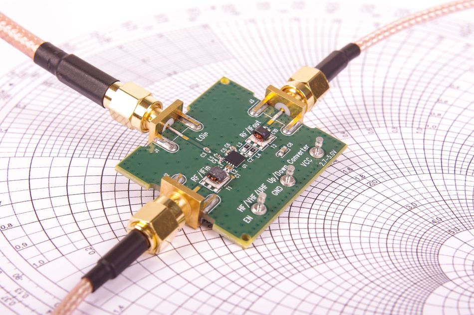
Controlled impedance is usually verified during PCB fabrication using test coupons and time-domain reflectometry (TDR). Measuring every signal trace on a finished board is often impractical because traces may be short, buried between layers, or inaccessible for probing. Instead, manufacturers use representative structures fabricated alongside the board to assess whether the process meets the specified impedance requirements.

What Is a Controlled-Impedance Test Coupon?

A test coupon is a small test structure manufactured on the same production panel as the PCB. It reproduces the relevant construction of the board, including the controlled-impedance layer, trace geometry, copper thickness, dielectric material, and reference-plane arrangement.

Coupons are commonly positioned near the edges of the production panel, although their number and placement depend on the manufacturer's process and the verification requirements. A panel may include coupons at different locations to help assess fabrication consistency.

An impedance coupon contains test traces designed to represent specific transmission-line structures on the PCB. Its geometry must correspond to the relevant board layers and target impedance. The manufacturer may also use separate coupons for other quality checks, such as copper plating, layer registration, or internal construction.

The coupon's reference-plane connections may be arranged to make measurement easier, even when those connections differ from the functional board. The important point is that the measured transmission-line structure must be suitable for representing the impedance being verified.

How Time-Domain Reflectometry Works

Time-domain reflectometry (TDR) measures impedance by sending a fast electrical step into a transmission line and observing the reflected signal. When the signal encounters a change in impedance, part of its energy is reflected toward the measurement instrument.

The reflection indicates that the line's impedance differs from the impedance expected by the incident signal. The magnitude and polarity of the reflection help determine the direction and size of the mismatch, while the time taken for the reflection to return helps locate the discontinuity along the line.

For a simple impedance discontinuity, the voltage reflection coefficient is:

Γ = (ZL - Z0) / (ZL + Z0)

Where:

• Γ = voltage reflection coefficient

• ZL = impedance at the discontinuity, in ohms (Ω)

• Z0 = characteristic impedance of the incident transmission line, in ohms (Ω)

A positive reflection indicates that the encountered impedance is higher than the line impedance; a negative reflection indicates that it is lower. The measured reflection can be used to estimate the impedance at the discontinuity, subject to the instrument's calibration and measurement conditions.

A TDR instrument converts the measured response into an impedance-versus-time or impedance-versus-distance display. This allows the manufacturer to assess whether the test structure remains within the specified impedance tolerance.

Measuring Single-Ended and Differential Impedance

Single-ended impedance is measured using a suitable TDR connection referenced to the appropriate return conductor. Differential impedance requires a measurement arrangement capable of evaluating the pair's differential response, typically using a differential TDR instrument or suitable differential test setup.

The test method must match the structure being verified. Trace geometry, probe or fixture connections, calibration, and the coupon's design can all affect the result.

What Does a Passing Coupon Prove?

A passing coupon indicates that the sampled test structure meets the agreed impedance acceptance criteria. Because it is manufactured alongside the PCB, it provides evidence that the relevant fabrication process is under control.

However, a passing coupon does not prove that every controlled-impedance trace on the finished board meets its target. Actual board routing may include vias, connectors, bends, layer transitions, and other discontinuities that are absent from the coupon. Coupon results should therefore be interpreted alongside the stackup, fabrication records, and any additional testing required by the design.

Before fabrication, the designer and PCB manufacturer should agree on the target impedance, tolerance, coupon configuration, measurement method, and reporting requirements. This ensures that the results provide meaningful evidence of compliance with the design specification.

Frequently Asked Questions About Controlled Impedance

What is controlled impedance in a PCB?

Controlled impedance is the design and fabrication of PCB traces to achieve a specified characteristic impedance within an agreed tolerance. It helps limit signal reflections and maintain signal integrity in high-speed digital, RF, and other transmission-line applications.

What is the difference between controlled impedance and characteristic impedance?

Characteristic impedance is an electrical property of a transmission line, determined by its geometry and surrounding materials. Controlled impedance is the design and manufacturing process used to achieve a target characteristic impedance within a specified tolerance.

Is 50 Ω or 100 Ω always required?

No. 50 Ω single-ended and 100 Ω differential are common targets, not universal requirements. The correct impedance depends on the interface specification, connected components, and system design.

What tolerance should I specify for controlled impedance?

The required tolerance depends on the interface, device specifications, and PCB manufacturer's capabilities. ±10% is common in PCB fabrication, but some designs require tighter limits, such as ±5%; confirm the acceptable range with the manufacturer before fabrication.

How is controlled impedance tested?

PCB manufacturers commonly use test coupons and time-domain reflectometry (TDR) to measure characteristic impedance. A fast electrical signal is applied to a representative transmission-line structure, and the reflected signal is analyzed to determine impedance variations along the line.

Does a passing test coupon guarantee every trace meets its target?

No. A passing coupon indicates that the sampled test structure meets the agreed acceptance criteria, but it does not directly verify every trace on the finished PCB. Actual board features, including vias, connectors, layer transitions, and routing discontinuities, may affect impedance and require separate evaluation.

References

[1] Analog Devices, “MT-094: Microstrip and Stripline Design,” Tutorial, Jan. 2009. [Online]. Available: https://www.analog.com/media/en/training-seminars/tutorials/MT-094.pdf. [Accessed: Oct. 20, 2026].

[2] IPC, “IPC-TM-650, Test Method 2.5.5.7A: Characteristic Impedance Lines on Printed Boards by TDR,” Mar. 2004. [Online]. Available: https://www.electronics.org/sites/default/files/test_methods_docs/2-5-5-7a.pdf. [Accessed: Oct. 20, 2026].

[3] Texas Instruments, “Layout Guidelines,” Application Brief SLLA653. [Online]. Available: https://www.ti.com/document-viewer/lit/html/SLLA653/GUID-A4F1CD83-9D39-45B1-B7A5-0E03429E4305. [Accessed: Oct. 20, 2026].

[4] Polar Instruments, “Controlled Impedance PCBs: An Introduction to the Design and Manufacture of Controlled Impedance PCBs.” [Online]. Available: https://www.polarinstruments.com/pdf/brochures/lit145.pdf. [Accessed: Oct. 20, 2026].

[5] Polar Instruments, “Controlled Impedance—Design for Test,” Application Note AP132. [Online]. Available: https://www.polarinstruments.com/support/cits/AP132.html. [Accessed: Oct. 20, 2026].

[6] Sierra Circuits, “Controlled Impedance Design Guide.” [Online]. Available: https://www.protoexpress.com/pcb-design-guides/controlled-impedance/. [Accessed: Oct. 20, 2026].

[7] Rogers Corporation, “RO4000 Series Laminates.” [Online]. Available: https://www.rogerscorp.com/advanced-electronics-solutions/ro4000-series-laminates/ro4003c-laminates. [Accessed: Oct. 20, 2026].