Audio event detection is the process of identifying specific sounds or patterns within an audio stream. From the subtle hum of a refrigerator to the distinct ring of a doorbell, this technology can pick out and categorize sounds with remarkable precision.

This article offers an in-depth exploration of audio event detection using a Particle Photon 2 device and Edge Impulse. We'll begin by demystifying the fundamentals of audio event detection through Edge artificial intelligence (AI), highlighting its importance, addressing its challenges, and showcasing its potential applications across diverse sectors.

Understanding Audio Event Detection

At its core, audio event detection is about differentiating between various sounds in an environment, be it the chirping of birds, the honking of cars, or the murmur of a distant conversation. The whole process of audio event detection can be broadly divided into the following steps:

1. Feature Extraction: Before any sound can be recognized, it needs to be transformed from a complex waveform into a set of features that can be more easily analyzed. This is done using techniques like Mel-frequency cepstral coefficients (MFCC)[1] or spectrograms. These techniques convert raw audio data into a representation that highlights its unique characteristics.

2. Model Training: Once features are extracted, they are used to train machine learning models. During this phase, the model is exposed to various audio samples and their corresponding labels (e.g., 'car honk', 'bird chirp'). Over time, the model learns to associate specific features with specific labels.

3. Real-time Detection: With a trained model in place, real-time audio event detection can commence. Incoming audio is continuously processed to extract features, which are then fed into the model. The model then predicts the most likely event or sound based on its training.

4. Post-processing: Sometimes, raw predictions from the model are further processed to improve accuracy. For instance, if a sound is transient (like a door slam), but the model detects it over a prolonged period, post-processing can correct such anomalies.

Applications of audio event detection

The transformative potential of audio event detection is vast, touching various sectors and reshaping how they operate. Here are some notable applications:

• Healthcare: Devices can analyze breathing patterns, helping in early detection of conditions like sleep apnea or asthma exacerbations. In assisted living facilities, audio event detection can identify sounds of distress or falls, ensuring timely assistance and potentially preventing serious injuries.

• Smart Homes: Homes can detect activities like reading, exercising, or cooking and adjust lighting, music or air conditioning accordingly. Beyond traditional alarms, systems can identify sounds of glass breaking or unfamiliar footsteps, alerting homeowners or security services.

• Environmental Monitoring: By recognizing specific animal calls, researchers can monitor species populations and migration patterns. Changes in natural soundscapes can indicate shifts in ecosystem health, such as dwindling insect populations or increased human encroachment.

• Transportation: Vehicles can analyze engine or machinery sounds to identify wear and tear, prompting maintenance before costly breakdowns occur. In public transport, unusual noises can trigger alerts, ensuring quick responses to potential issues.

• Entertainment: Home entertainment systems can adjust volume or switch to a clearer audio channel based on ambient noise levels. In theaters, real-time reactions (like laughter or applause) can be analyzed to adjust pacing or volume for an optimal experience.

• Defense: Advanced systems can differentiate between routine and suspicious sounds, from the hum of a drone to hushed conversations, providing crucial intelligence. On borders or in conflict zones, audio event detection can identify vehicle movements, weapon discharges, or other potential threats, enabling rapid response.

Having explored the vast applications of audio event detection, one might wonder about the technological mechanisms and platforms that empower these applications to function with such precision and efficiency. How do these systems accurately identify and categorize a vast array of sounds in real-time?

The next section introduces a feature-rich Internet of Things (IoT) platform, which, when combined with appropriate Edge AI tools, becomes a versatile solution for deploying various audio event detection applications.

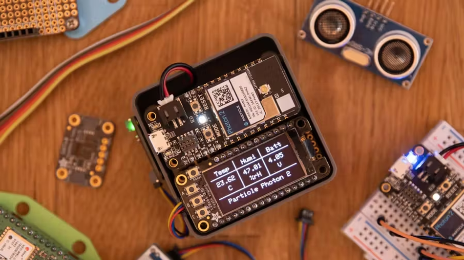
Particle Photon 2

When it comes to picking the right IoT platform for applications like audio event recognition, Particle Photon 2 stands out. The integration of the ARM Cortex M33 microcontroller provides the computational capability required for processing audio data in real-time, a critical factor for audio event detection.

Fig. 1: The Particle Photon 2 module. Source: Hackster.io

Its design facilitates cloud connectivity, enabling functionalities such as over-the-air updates, real-time data monitoring, and remote diagnostics, all of which can be pivotal when dealing with dynamic audio patterns in IoT projects. The Particle Photon 2 offers a comprehensive set of tools, libraries, and integrations, designed to streamline both the prototyping and scaling processes for audio-based applications. 

With security being paramount, especially when transmitting audio data, it incorporates encrypted communication protocols and secure boot mechanisms. The growing community around Particle provides a collaborative platform for developers, especially those focusing on audio applications. 

When paired with platforms like Edge Impulse, the Particle Photon 2 is positioned to leverage machine learning capabilities at the edge, optimizing audio data collection, model training, and deployment. 

Let’s now take a look at a tutorial explaining how to implement audio event detection with Particle Photon 2.

Audio Event Detection with Particle Boards

In this tutorial, you'll use machine learning to build a model that recognizes when a doorbell rings. You'll use the Particle Photon 2, a microphone, a cell phone, and Edge Impulse to build this project. You can add the ability to send an SMS message when the doorbell rings by following the tutorial on Particle's website.

Audio event detection is a common machine learning task, and is a hard task to solve using rule-based programming. You'll learn how to collect audio data, build a neural network classifier, and how to deploy your model back to a device. At the end of this tutorial, you'll have a firm understanding of applying machine learning on Particle hardware using Edge Impulse.

Before starting the tutorial

After signing up for a free Edge Impulse account, clone the finished project, including all training data, signal processing and machine learning blocks here: Particle - Doorbell. At the end of the process you will have the full project that comes pre-loaded with training and test datasets.

1. Prerequisites

For this tutorial you'll need the:

• Particle Photon2 Board with the Edge ML Kit.

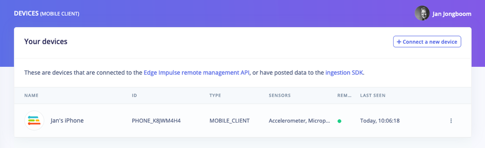
Before starting ingestion create an Edge Impulse account if you haven't already. To collect audio data you can use any mobile phone. Follow in the instructions on that page to connect your phone to your Edge Impulse project.

Once your device is connected under Devices in the studio you can proceed:

Connected devices

2. Collecting your first data

To build this project, you'll need to collect some audio data that will be used to train the machine learning model. Since the goal is to detect the sound of a doorbell, you'll need to collect some examples of that. You'll also need some examples of typical background noise that doesn't contain the sound of a doorbell, so the model can learn to discriminate between the two. These two types of examples represent the two classes we'll be training our model to detect: unknown noise, or doorbell.

Your phone will show up like any other device in Edge Impulse, and will automatically ask permission to use sensors. Let's start by recording an example of background noise that doesn't contain the sound of a doorbell. On your cell set the label to unknown, the sample length to 2 seconds. This indicates that you want to record 1 second of audio, and label the recorded data as unknown. You can later edit these labels if needed.

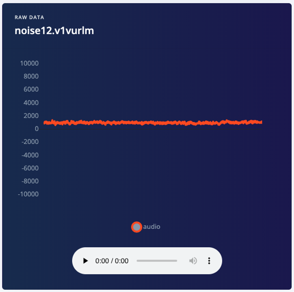
After you click Start recording, the device will capture a second of audio and transmit it to Edge Impulse.

When the data has been uploaded, you will see a new line appear under 'Collected data' in the Data acquisition tab of your Edge Impulse project. You will also see the waveform of the audio in the 'RAW DATA' box. You can use the controls underneath to listen to the audio that was captured.

Audio waveform

Machine learning works best with lots of data, so a single sample won't cut it. Now is the time to start building your own dataset. For example, use the following two classes, and record around 3 minutes of data per class:

• doorbell - Record yourself ringing the doorbell in the same room

• unknown - Record the background noise in your house

3. Designing an impulse

With the training set in place you can design an impulse. An impulse takes the raw data, slices it up in smaller windows, uses signal processing blocks to extract features, and then uses a learning block to classify new data. Signal processing blocks always return the same values for the same input and are used to make raw data easier to process, while learning blocks learn from past experiences.

For this tutorial we'll use the signal processing block. Then we'll use a 'Neural Network' learning block, that takes these generated features and learns to distinguish between our different classes (circular or not).

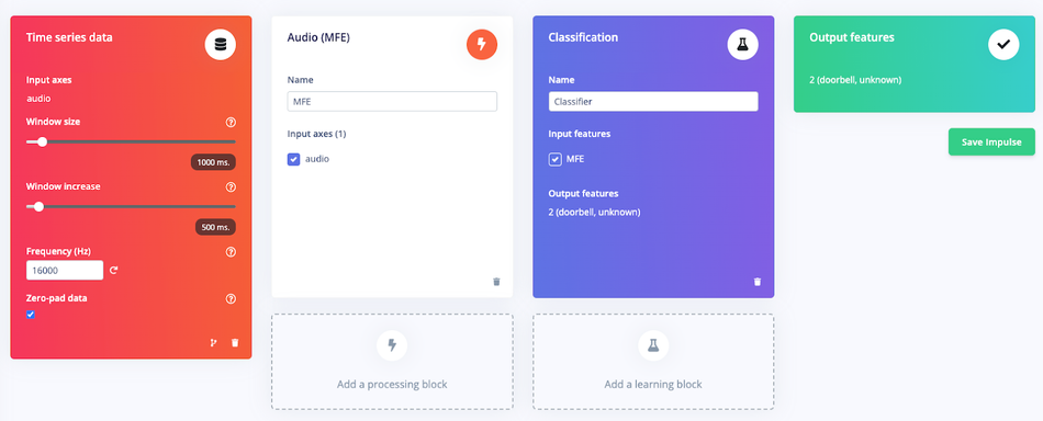
In the studio go to Create impulse, set the window size to 1000 (you can click on the 1000 ms. text to enter an exact value), the window increase to 500, and add the 'Audio MFCC' and 'Classification (Keras)' blocks. Then click Save impulse.

Impulse with processing and learning blocks

Configuring the MFCC block

Now that we've assembled the building blocks of our Impulse, we can configure each individual part. Click on the MFCC tab in the left hand navigation menu. You'll see a page that looks like this:The MFCC page.

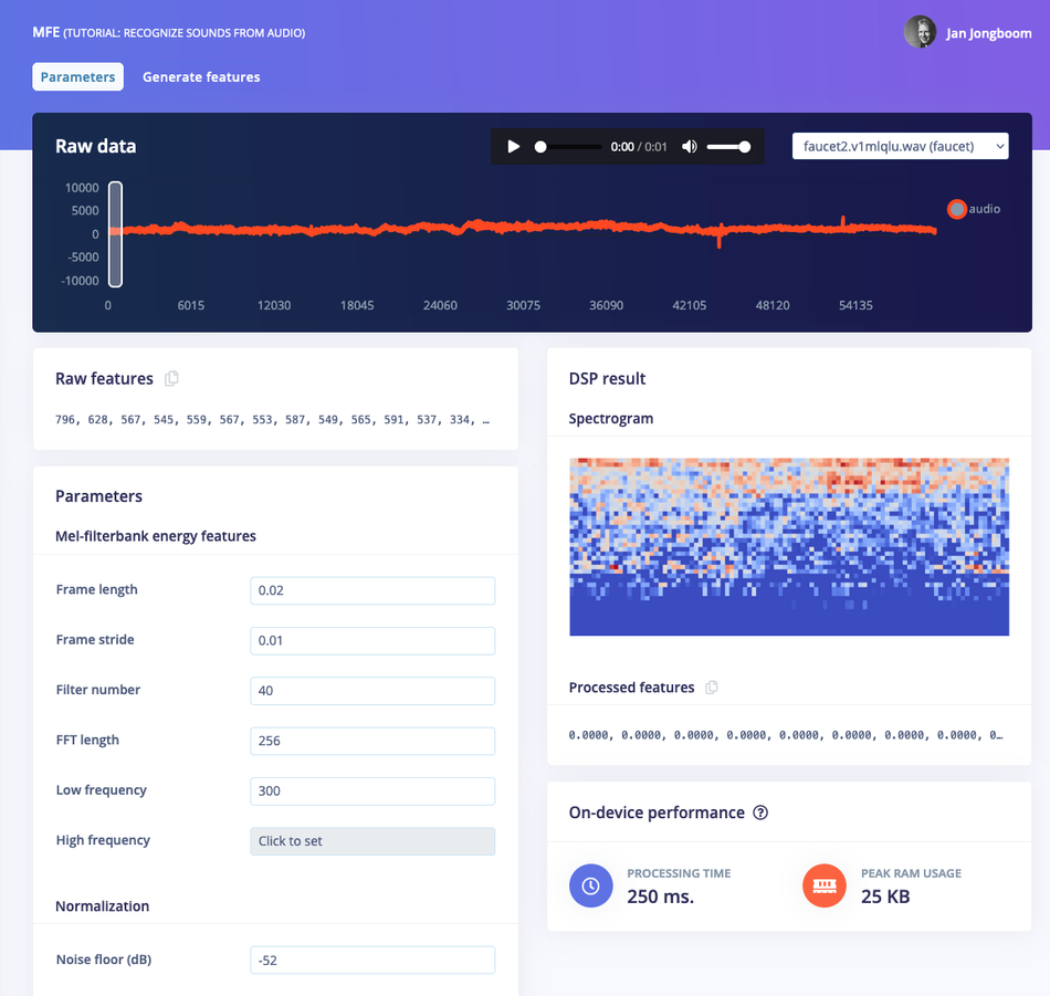
This page allows you to configure the MFCC block, and lets you preview how the data will be transformed. The right of the page shows a visualization of the MFCC's output for a piece of audio, which is known as a spectrogram.

The MFCC block transforms a window of audio into a table of data where each row represents a range of frequencies and each column represents a span of time. The value contained within each cell reflects the amplitude of its associated range of frequencies during that span of time. The spectrogram shows each cell as a colored block, the intensity which varies depends on the amplitude.

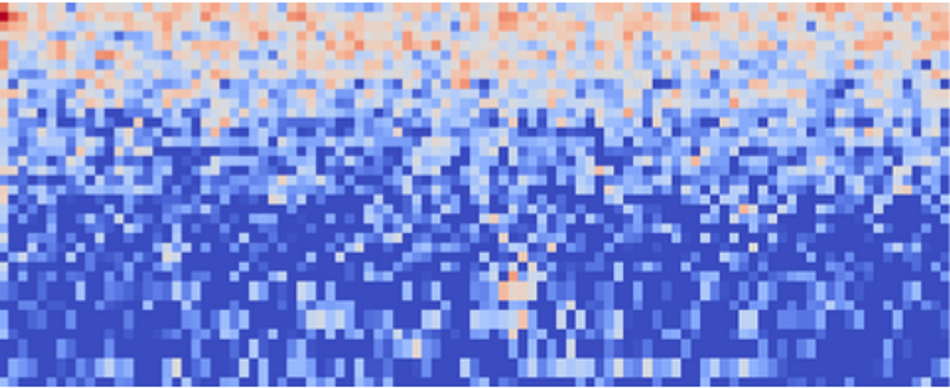
The patterns visible in a spectrogram contain information about what type of sound it represents. For example, the spectrogram in this image shows a pattern typical of background noise:Spectrogram of background noise.

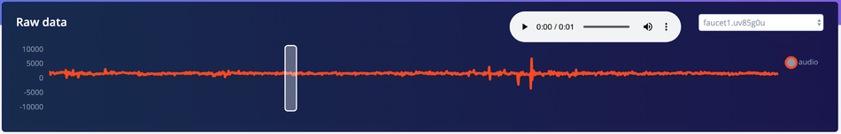
It's interesting to explore your data and look at the types of spectrograms it results in. You can use the dropdown box near the top right of the page to choose between different audio samples to visualize, and drag the white window on the audio waveform to select different windows of data:Audio waveform and sample dropdown box.

There are a lot of different ways to configure the MFCC block, as shown in the Parameters box:

The MFCC parameters box.

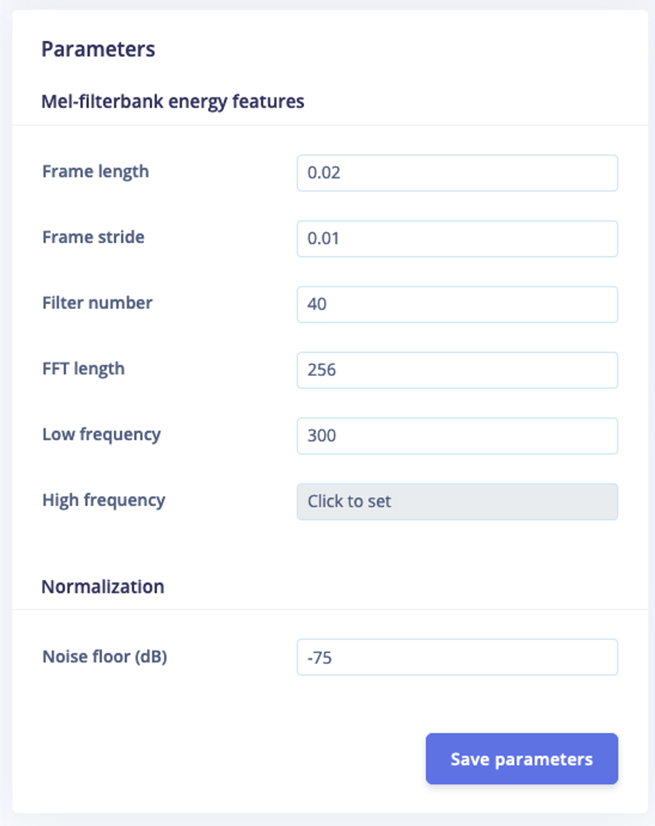
Handily, Edge Impulse provides sensible defaults that will work well for many use cases, so we can leave these values unchanged. You can play around with the noise floor to quickly see the effect it has on the spectrogram.

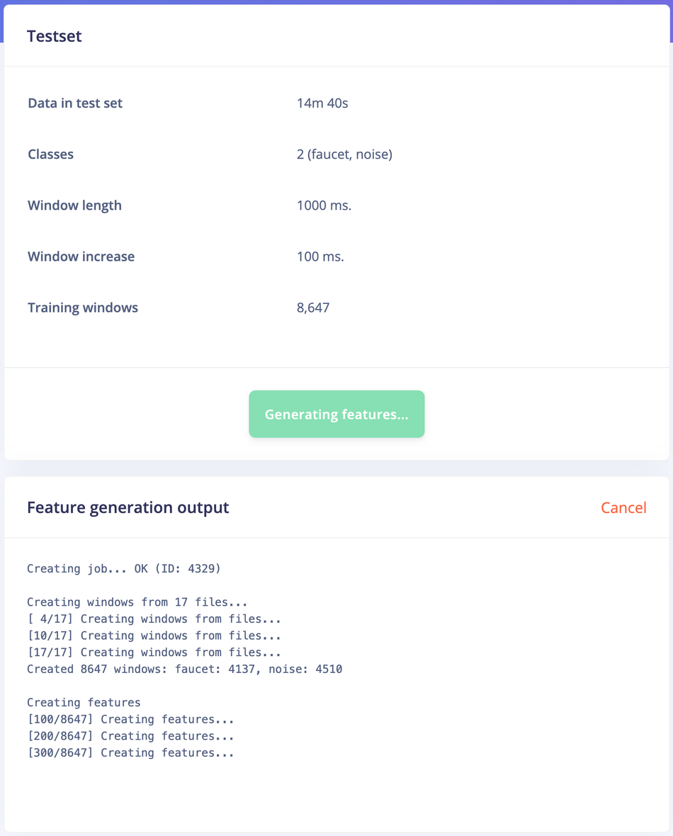
The spectrograms generated by the MFCC block will be passed into a neural network architecture that is particularly good at learning to recognize patterns in this type of tabular data. Before training our neural network, we'll need to generate MFCC blocks for all of our windows of audio. To do this, click the Generate features button at the top of the page, then click the green Generate features button. If you have a full 10 minutes of data, the process will take a while to complete:Running the feature generation process.

Once this process is complete the feature explorer shows a visualization of your dataset. Here dimensionality reduction is used to map your features onto a 3D space, and you can use the feature explorer to see if the different classes separate well, or find mislabeled data (if it shows in a different cluster). You can find more information in visualizing complex datasets.

Next, we'll configure the neural network and begin training.

Configuring the neural network

With all data processed it's time to start training a neural network. Neural networks are algorithms, modeled loosely after the human brain, that can learn to recognize patterns that appear in their training data. The network that we're training here will take the MFCC as an input, and try to map this to one of two classes—doorbell or unknown.

Click on NN Classifier in the left hand menu. You'll see the following page:The NN Classifier page.

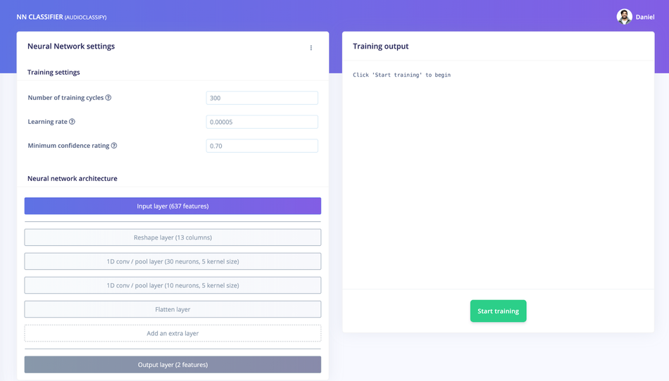
A neural network is composed of layers of virtual "neurons", which you can see represented on the left hand side of the NN Classifier page. An input—in our case, an MFCC spectrogram—is fed into the first layer of neurons, which filters and transforms it based on each neuron's unique internal state. The first layer's output is then fed into the second layer, and so on, gradually transforming the original input into something radically different. In this case, the spectrogram input is transformed over four intermediate layers into just two numbers: the probability that the input represents noise, and the probability that the input represents a doorbell.

During training, the internal state of the neurons is gradually tweaked and refined so that the network transforms its input in just the right ways to produce the correct output. This is done by feeding in a sample of training data, checking how far the network's output is from the correct answer, and adjusting the neurons' internal state to make it more likely that a correct answer is produced next time. When done thousands of times, this results in a trained network.

A particular arrangement of layers is referred to as an architecture, and different architectures are useful for different tasks. The default neural network architecture provided by Edge Impulse will work well for our current project, but you can also define your own architectures. You can even import custom neural network code from tools used by data scientists, such as TensorFlow and Keras.

The default settings should work, and to begin training, click Start training. You'll see a lot of text flying past in the Training output panel, which you can ignore for now. Training will take a few minutes. When it's complete, you'll see the Model panel appear at the right side of the page.

Congratulations, you've trained a neural network with Edge Impulse! But what do all these numbers mean?

At the start of training, 20% of the training data is set aside for validation. This means that instead of being used to train the model, it is used to evaluate how the model is performing. The Last training performance panel displays the results of this validation, providing some vital information about your model and how well it is working. Bear in mind that your exact numbers may differ from the ones in this tutorial.

On the left hand side of the panel, Accuracy refers to the percentage of windows of audio that were correctly classified. The higher number the better, although an accuracy approaching 100% is unlikely, and is often a sign that your model has overfit the training data. You will find out whether this is true in the next stage, during model testing. For many applications, an accuracy above 80% can be considered very good.

The Confusion matrix is a table showing the balance of correctly versus incorrectly classified windows. To understand it, compare the values in each row.

The On-device performance region shows statistics about how the model is likely to run on-device. Inferencing time is an estimate of how long the model will take to analyze one second of data on a typical microcontroller (here: an Arm Cortex-A33 running at 200MHz). Peak memory usage gives an idea of how much RAM will be required to run the model on-device.

4. Classifying new data

The performance numbers in the previous step show that our model is working well on its training data, but it's extremely important that we test the model on new, unseen data before deploying it in the real world. This will help us ensure the model has not learned to overfit the training data, which is a common occurrence.

Edge Impulse provides some helpful tools for testing our model, including a way to capture live data from your device and immediately attempt to classify it. To try it out, click on Live classification in the left hand menu. Your device should show up in the 'Classify new data' panel. Capture 5 seconds of background noise by clicking Start sampling.

The sample will be captured, uploaded, and classified. Once this has happened, you'll see a breakdown of the results.

Once the sample is uploaded, it is split into windows–in this case, a total of 41. These windows are then classified. As you can see, our model classified all 41 windows of the captured audio as noise. This is a great result! Our model has correctly identified that the audio was background noise, even though this is new data that was not part of its training set.

Of course, it's possible some of the windows may be classified incorrectly. If your model didn't perform perfectly, don't worry. We'll get to troubleshooting later.

Misclassifications and uncertain results

It's inevitable that even a well-trained machine learning model will sometimes misclassify its inputs. When you integrate a model into your application, you should take into account that it will not always give you the correct answer.

For example, if you are classifying audio, you might want to classify several windows of data and average the results. This will give you better overall accuracy than assuming that every individual result is correct.

5. Model testing

Using the Live classification tab, you can easily try out your model and get an idea of how it performs. But to be really sure that it is working well, we need to do some more rigorous testing. That's where the Model testing tab comes in. If you open it up, you'll see the sample we just captured listed in the Test data panel.

In addition to its training data, every Edge Impulse project also has a test dataset. Samples captured in Live classification are automatically saved to the test dataset, and the Model testing tab lists all of the test data.

To use the sample we've just captured for testing, we should correctly set its expected outcome. Click the ⋮ icon and select Edit expected outcome, then enter noise. Now, select the sample using the checkbox to the left of the table and click Classify selected.

You'll see that the model's accuracy has been rated based on the test data. Right now, this doesn't give us much more information that just classifying the same sample in the Live classification tab. But if you build up a big, comprehensive set of test samples, you can use the Model testing tab to measure how your model is performing on real data.

Ideally, you'll want to collect a test set that contains a minimum of 25% the amount of data of your training set. So, if you've collected 10 minutes of training data, you should collect at least 2.5 minutes of test data. You should make sure this test data represents a wide range of possible conditions, so that it evaluates how the model performs with many different types of inputs. For example, collecting test audio for several different doorbells, perhaps moving collecting the audio in a different room, is a good idea.

You can use the Data acquisition tab to manage your test data. Open the tab, and then click Test data at the top. Then, use the Record new data panel to capture a few minutes of test data, including audio for both background noise and doorbells. Make sure the samples are labelled correctly. Once you're done, head back to the Model testing tab, select all the samples, and click Classify selected.

The screenshot shows classification results from a large number of test samples (there are more on the page than would fit in the screenshot). It's normal for a model to perform less well on entirely fresh data.

For each test sample, the panel shows a breakdown of its individual performance. Samples that contain a lot of misclassifications are valuable, since they have examples of types of audio that our model does not currently fit. It's often worth adding these to your training data, which you can do by clicking the ⋮ icon and selecting Move to training set. If you do this, you should add some new test data to make up for the loss!

Testing your model helps confirm that it works in real life, and it's something you should do after every change. However, if you often make tweaks to your model to try to improve its performance on the test dataset, your model may gradually start to overfit to the test dataset, and it will lose its value as a metric. To avoid this, continually add fresh data to your test dataset.

Data hygiene

It's extremely important that data is never duplicated between your training and test datasets. Your model will naturally perform well on the data that it was trained on, so if there are duplicate samples then your test results will indicate better performance than your model will achieve in the real world.

6. Model troubleshooting

If the network performed great, fantastic! But what if it performed poorly? There could be a variety of reasons, but the most common ones are:

1. The data does not look like other data the network has seen before. This is common when someone uses the device in a way that you didn't add to the test set. You can add the current file to the test set by adding the correct label in the 'Expected outcome' field, clicking ⋮, then selecting Move to training set.

2. The model has not been trained enough. Increase number of epochs to 200 and see if performance increases (the classified file is stored, and you can load it through 'Classify existing validation sample').

3. The model is overfitting and thus performs poorly on new data. Try reducing the number of epochs, reducing the learning rate, or adding more data.

4. The neural network architecture is not a great fit for your data. Play with the number of layers and neurons and see if performance improves.

As you see, there is still a lot of trial and error when building neural networks. Edge Impulse is continually adding features that will make it easier to train an effective model.

7. Deploying to your device

With the impulse designed, trained and verified you can deploy this model back to your device. This makes the model run without an internet connection, minimizes latency, and runs with minimum power consumption.

To export your model, click on Deployment in the menu. Then under 'Build firmware' select the Particle Library.

8. Flashing the device

Once optimized parameters have been found, you can click Build. This will build a particle workbench compatible package that will run on your development board. After building is completed you'll get prompted to download a zipfile. Save this on your computer. A pop-up video will show how the download process works.

After unzipping the downloaded file, you can open the project in Particle Workbench.

Flash a Particle Photon 2 Project

The development board does not come with the Edge Impulse firmware. To flash the Edge Impulse firmware:

1. Open a new VS Code window, ensure that Particle Workbench has been installed (see above)

2. Use VS Code Command Palette and type in Particle: Import Project

   1. Select the project.properties file in the directory that you just downloaded and extracted from the section above.

3. Use VS Code Command Palette and type in Particle: Configure Project for Device

   1. Select deviceOS@5.3.2 (or a later version)

   2. Choose a target. (e.g. P2 , this option is also used for the Photon 2).

4. It is sometimes needed to manually put your Device into DFU Mode. You may proceed to the next step, but if you get an error indicating that "No DFU capable USB device available" then please follow these step.

   1. Hold down both the RESET and MODE buttons.

   2. Release only the RESET button, while holding the MODE button.

   3. Wait for the LED to start flashing yellow.

   4. Release the MODE button.

5. Compile and Flash in one command with: Particle: Flash application & DeviceOS (local)

Local Compile Only! At this time you cannot use the Particle: Cloud Compile or Particle: Cloud Flash options; local compilation is required.

Serial Connection to Computer

The Particle libraries generated by Edge Impulse have serial output through a virtual COM port on the serial cable. The serial settings are 115200, 8, N, 1. Particle Workbench contains a serial monitor accessible via Particle: Serial Monitor via the VS Code Command Palette.

Device compatibility

Initial release of the particle integration will rely on the particle-ingestion project and the data forwarder to be installed on the device and computer. This is currently only supported on the Particle Photon 2, but should run on other devices as well.

Stand Alone Example with Static Buffer

This standalone example project contains minimal code required to run the imported impulse on the E7 device. This code is located in main.cpp. In this minimal code example, inference is run from a static buffer of input feature data. To verify that our embedded model achieves the exact same results as the model trained in Studio, we want to copy the same input features from Studio into the static buffer in main.cpp.

To do this, first head back to Edge Impulse Studio and click on the Live classification tab. Follow this video for instructions.

In main.cpp paste the raw features inside the static const float features[] definition, for example:

static const float features[] = {
-19.8800, -0.6900, 8.2300, -17.6600, -1.1300, 5.9700, ...
};

The project will repeatedly run inference on this buffer of raw features once built. This will show that the inference result is identical to the Live classification tab in Studio. Use new sensor data collected in real time on the device to fill a buffer. From there, follow the same code used in main.cpp to run classification on live data.

Running the model on the device

Follow the flashing instructions above to run on device.

Victory! You've now built your first on-device machine learning model.

7. Conclusion

Congratulations! Now that you've trained and deployed your model you can go further and build your own custom firmware. We can't wait to see what you'll build! 🚀

Future Trends and Developments in Audio Event Detection

As we delve deeper into the era of smart technologies and AI, audio event detection is set to undergo transformative changes that will not only refine its existing framework but also introduce novel approaches to audio signal processing and analysis.

The upcoming phase in audio event detection technology is expected to be characterized by a synergy of enhanced algorithms, deep learning models, and sophisticated hardware designs. These elements will work in tandem to offer solutions that are not only precise but also adaptable to the dynamic auditory environments we encounter daily. Here are some trends and developments that are anticipated to shape the future of audio event detection:

• Advanced Signal Processing & Feature Extraction: Future algorithms will be more refined, capable of extracting salient features from audio signals with unprecedented accuracy. New feature extraction techniques will emerge, capturing the subtleties and nuances of various audio events, providing a richer dataset for model training and inference.

• Deep Learning and Adaptive Models: The incorporation of deep learning and adaptive models will revolutionize the detection process. These models will not only understand complex audio patterns but also learn and adapt to environmental changes in real-time, ensuring consistent performance and reliability over time.

• Edge AI and Hardware Acceleration: With devices like Particle Photon 2 leading the charge, the future will see significant improvements in Edge AI. Enhanced on-device processing capabilities, backed by hardware accelerators for AI, will facilitate swift, real-time decision-making and detection, even in environments with limited connectivity.

• Energy Efficiency and Sustainable Designs: Sustainability will be at the forefront, with the development of energy-efficient hardware and software designs. These designs will be crucial for devices deployed in remote areas, ensuring longevity and reducing the need for frequent maintenance or battery replacements.

• Security, Standardization, and Interoperability: As the technology becomes more widespread, there will be an increased focus on security and standardization. Advanced encryption techniques will safeguard data privacy, while standardization efforts will ensure seamless interoperability between various devices and platforms in the audio event detection ecosystem.

Conclusion

The impending advancements in audio event detection technology herald a future where devices are not only more accurate but also more intelligent and autonomous. With a combination of sophisticated algorithms, adaptive learning models, and robust hardware, the next generation of audio event detection is poised to seamlessly integrate into diverse applications, providing reliable and efficient solutions for various challenges in the auditory landscape.

About the sponsor: Edge Impulse

Edge Impulse is the leading development platform for embedded machine learning, used by over 1,000 enterprises across 200,000 ML projects worldwide. We are on a mission to enable the ultimate development experience for machine learning on embedded devices for sensors, audio, and computer vision, at scale. 

From getting started in under five minutes to MLOps in production, we enable highly optimized ML deployable to a wide range of hardware from MCUs to CPUs, to custom AI accelerators. With Edge Impulse, developers, engineers, and domain experts solve real problems using machine learning in embedded solutions, speeding up development time from years to weeks. We specialize in industrial and professional applications including predictive maintenance, anomaly detection, human health, wearables, and more.

References

[1] Z. K. Abdul and A. K. Al-Talabani, "Mel Frequency Cepstral Coefficient and its Applications: A Review," in IEEE Access, vol. 10, pp. 122136-122158, 2022, doi: 10.1109/ACCESS.2022.3223444.