Optimizing Machine Learning Models for Resource-Constrained Embedded Devices
Article #5 of Confronting AI Series: Smart ML on embedded systems demands efficiency under tight memory, compute, and latency constraints. Techniques like pruning, quantization, low-rank decomposition, and federated learning enable compact, fast, and reliable models for edge intelligence.

30 Jul, 2025. 11 minutes read

This is the fifth article in our multi-part Confronting AI series, brought to you by Mouser Electronics. Based on the Methods: Confronting AI e-magazine, this series explores how artificial intelligence is reshaping engineering, product design, and the ethical frameworks behind emerging technologies. Each article examines real-world opportunities and unresolved tensions—from data centers and embedded ML to regulation, adoption, and ethics. Whether you're developing AI systems or assessing their broader impact, the series brings clarity to this rapidly evolving domain.

"AI Everywhere" explains how AI extends beyond LLMs into vision, time series, ML, and RL.
"The Paradox of AI Adoption" focuses on trust and transparency challenges in AI adoption.
“Repowering Data Centers for AI” explores powering data centers sustainably for AI workloads.
“Revisiting AI’s Ethical Dilemma” revisits ethical risks and responsible AI deployment.
“Overcoming Constraints for Embedded ML” presents ways to optimize ML models for embedded systems.
“The Regulatory Landscape of AI” discusses AI regulation and balancing safety with innovation.
Embedded systems are increasingly incorporating machine learning (ML) to enable smart and autonomous functionalities. However, implementing ML on these devices presents unique challenges due to their inherent resource constraints. Unlike general-purpose systems such as desktops or cloud servers, embedded systems are often battery-powered, operate with limited memory and processing capabilities, and interact with sensor-based data like time-varying analog signals. These differences demand innovative solutions to overcome issues like limited computational resources, small and noisy datasets, and strict real-time requirements. This article explores a range of optimization techniques and model design strategies that enable effective ML on embedded devices, ensuring that these systems remain efficient, reliable, and capable of meeting application-specific demands.
Recommended reading: Bringing Intelligence to the Edge Series
Understanding the Challenges
As an engineer or developer working with embedded systems, your role is crucial in overcoming the unique challenges of implementing ML technologies. Unlike generative artificial intelligence (AI) applications accessed from personal computers, which primarily use text prompts, edge devices process sensor outputs, which are analog signals of time-varying voltage or current. In addition to this difference in training and inference data, computational resources and data constraints are also key challenges to using edge-based ML systems.
Limited Computational Resources
Memory, processing power, and battery life are often limited, necessitating lightweight models and efficient computation techniques. Microcontrollers typically feature specifications measured in megahertz and megabytes, whereas desktops and servers are measured in gigahertz and gigabytes.
Data Constraints
Small datasets, noisy data, and limited access to diverse data sources should be expected. These factors increase the risk of overfitting and require robust methods to improve generalization. Overfitting can result in poor generalization, meaning the system performs poorly (e.g., incorrect predictions) in real-world conditions. It can also consume more memory and compute cycles, potentially resulting in poor energy efficiency.
Many embedded systems demand low-latency inferencing, which requires efficient models capable of delivering predictions within strict time constraints. Failing to meet these requirements can result in a system response that appears sluggish to the end user. Human factors research teaches us that 100 to 300 milliseconds is considered acceptable for an instantaneous response. This underscores the importance of designing models that can meet these real-world demands.
Model Optimization Techniques
Striking the right balance between model size and complexity, from a memory perspective, while ensuring accurate predictions during inferencing is challenging. Making the model too small can compromise its prediction ability, while training the model to account for nearly all possible inputs can make it too large to fit in the limited memory space of a microcontroller. Achieving this balance is crucial and can be done using a variety of techniques.
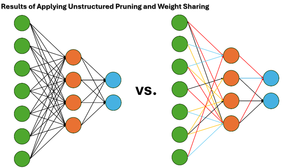
Weight Sharing
A weight-sharing technique reduces the number of parameters in a model, making it smaller and more efficient. Instead of assigning unique weights to each connection in the network, similar neurons share the same weights. For example, in image processing tasks, weight sharing ensures that the same features—measurable variables like edges or textures—are detected across the entire image rather than learning separate weights for each region. This reduces the model's parameter count and improves generalization by leveraging the fact that features in one part of an image are often relevant to others.
Model Pruning
Model pruning involves removing unnecessary neurons or layers from neural networks to reduce computational and memory overhead. Pruning is broadly categorized as structured and unstructured.
Structured pruning removes entire neurons, channels, or layers while maintaining dense matrices, making it more compatible with standard hardware. Common structured approaches include channel pruning (remove less critical channels in convolutional layers), layer pruning (remove redundant layers, especially in deeper networks), and group-wise pruning (target specific groups of neurons or filters).
Unstructured pruning removes individual weights (connections) with low importance, such as those with a weight close to zero (Figure 1). This pruning results in sparse matrices requiring specialized libraries or hardware for efficient computation, as irregular sparsity may lead to inefficiencies on general-purpose hardware.
Quantization
Quantization converts high-precision weights (e.g., 32-bit) to lower precision (e.g., 8-bit or even binary precision) and can save memory and speed computation using hardware accelerators. One method is post-training quantization, which quantifies a pre-trained floating-point model without retraining. A variant of the post-training method—dynamic range quantization—quantizes weights to lower precision, but activations remain as floating-point numbers during inference. Another variant is full integer quantization, wherein both weights and activations are quantized to integers.
Another method is quantization-aware training (QAT), which incorporates quantization during the training process. This simulates low-precision computation during training to minimize the impact on accuracy.
Overfitting Mitigation
Overfitting refers to an ML model that performs exceptionally well on training data but poorly on unseen data. Mitigation methods include augmentation, which expands the dataset to improve generalization by generating transformed versions of existing samples (e.g., rotating images). For sensor data acquired by embedded systems—typically time series data—techniques such as window slicing, jittering, and time warping introduce variations in sequential data that are useful in mitigating overfitting.
Other techniques, such as L1/L2 regularization, reduce overfitting by penalizing large weights. L1 regularization adds the sum of the absolute values of the weights, encouraging sparsity by driving less important weights to zero, which can also serve as a form of feature selection. L2 regularization adds the sum of the squared weights, discouraging large weights and promoting smoothness in the model by spreading influence across all features. The dropout technique randomly removes neurons during training and prevents overreliance on specific network pathways.
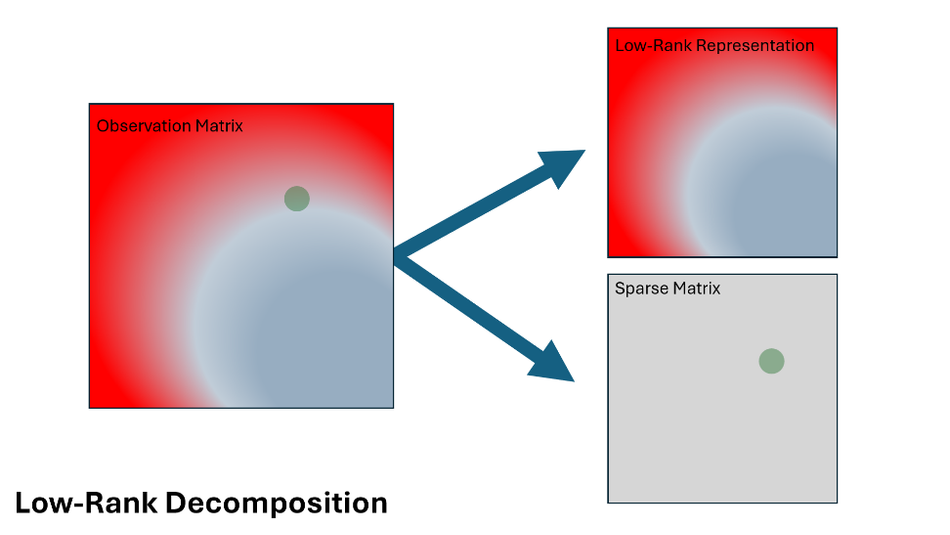
Low-Rank Decomposition
Low-rank decomposition reduces ML models' computational and memory demands by breaking down large-weight matrices into smaller, simpler matrices (Figure 2). In a typical neural network, weight matrices can be huge, consuming substantial memory and processing power. Low-rank decomposition approximates these large matrices as the product of two or more smaller matrices, requiring fewer parameters to store and manipulate. This decomposition significantly reduces the number of operations required during forward and backward passes, speeding up inference and training.
Efficient Loss Functions
A loss function is a mathematical formula that measures how far the model's predictions are from the actual values. It guides the training process to improve performance. Such functions include binary cross-entropy, mean squared error (MSE), and hinge loss.
Binary Cross-Entropy
This loss function is commonly used for binary classification tasks, where the goal is to classify data into two categories (e.g., "yes" or "no," "cat" or "dog"). It is particularly efficient and effective for low-complexity models because it directly measures the accuracy of probability-based predictions, ensuring the model learns to distinguish between the two classes accurately.
Mean Squared Error
Often applied to regression tasks, where the objective is to predict continuous values (like house prices or temperature), MSE calculates the average squared difference between predicted and actual values. This method is computationally lightweight and straightforward, making it a practical choice for resource-constrained environments.
Hinge Loss
This loss function is used with support vector machines (SVMs), a type of model designed for classification tasks. Hinge loss creates a margin around the decision boundary, ensuring predictions fall confidently on one side of the boundary. It is particularly effective for smaller datasets and simpler embedded systems, where computational efficiency and robust classification are priorities.
Additional Techniques for Optimizing ML Models for Embedded Systems
In addition to the previous methods, the following techniques help embedded designers further optimize ML models.
Feature Engineering and Selection
Effectively engineering and selecting features can drastically simplify a model while reducing computational and memory requirements. The model can achieve better performance with fewer resources by focusing on the most relevant information.
Feature Importance Analysis
This process involves identifying which features significantly impact the model’s predictions. By prioritizing these critical features and discarding irrelevant ones, the model becomes more efficient and accurate. For example, focusing on weather trends in a temperature monitoring system may outweigh less relevant data like timestamps.
Dimensionality Reduction
Techniques like principal component analysis (PCA) and t-distributed stochastic neighbor embedding (t-SNE) reduce the number of input features by summarizing or compressing data while retaining their essential characteristics. This minimizes memory and computational requirements, making the model faster and lighter, which is ideal for embedded systems.
Hyperparameter Tuning
Adjusting hyperparameters—the settings that control how a model learns—can significantly impact the model's efficiency and accuracy, especially on resource-constrained embedded devices.
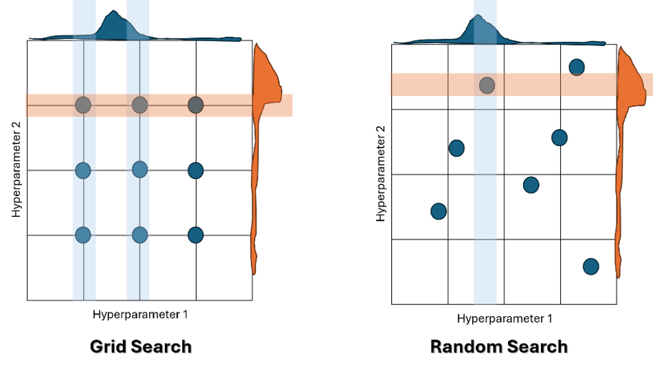
Random Search and Grid Search
Random search is a hyperparameter tuning technique where combinations of hyperparameters are sampled randomly within specified ranges. Unlike grid search, which evaluates all possible combinations, random search explores the parameter space more efficiently, often finding optimal or near-optimal settings with fewer evaluations (Figure 3). This efficiency makes it especially useful in embedded systems, where computational resources and time are limited, enabling faster tuning and reduced overhead.
Bayesian Optimization
Bayesian optimization is a more sophisticated approach that iteratively refines the search for optimal hyperparameters. Using prior evaluations to guide the next set of experiments, this strategy can reduce the need for computationally expensive exhaustive searches, making it especially beneficial for embedded systems.
Optimization Algorithms
Efficient optimization algorithms are critical to accelerating model convergence and minimizing resource consumption during training.
Gradient Descent
Variants of gradient descent optimization, such as stochastic gradient descent (SGD), Adam, and RMSprop, provide different trade-offs in terms of convergence speed, stability, and memory requirements. For instance, the Adam algorithm is widely used for its adaptive learning rates, making it robust and efficient for embedded ML.
Adaptive Optimization
Algorithms such as AdaGrad and Adam dynamically adjust the learning rate during training. This adaptability helps models converge faster with fewer iterations, saving computational resources—an essential consideration for embedded systems.
Model Training
Training an ML model from scratch can be computationally expensive, time-consuming, and often impractical for embedded systems. Leveraging pre-trained models and advanced training strategies can significantly reduce the workload.
Fine-Tuning
Instead of building a model from the ground up, fine-tuning involves adjusting specific layers of a pre-trained model. This approach customizes the model for a particular task while conserving resources.
Transfer Learning
This technique uses pre-trained models developed for similar tasks, significantly reducing the computational cost of training. For example, a model trained for object recognition can be adapted for specific objects on an embedded device, saving both time and energy.
Federated Learning
The model is trained across multiple devices without transferring raw data to a central server. This approach reduces network demands, preserves user privacy, and enables distributed training, making it an excellent fit for edge and embedded systems.
Hardware-Aware Model Design
Designing models with hardware specifications in mind maximizes efficiency and performance.
Neural architecture search (NAS): NAS techniques automatically design models optimized for specific hardware, balancing accuracy and computational requirements.
Hardware acceleration: Leveraging specialized hardware like graphics processing units (GPUs), tensor processing units (TPUs), or neural processing units (NPUs) can accelerate training and inference, crucial for power and time efficiency on embedded devices.
Recommended reading: TPU vs GPU in AI
Hardware-tailored frameworks: Leveraging frameworks tailored to specific hardware platforms, such as TensorFlow Lite, ONNX Runtime, or Edge Impulse, can optimize inference performance on supported embedded hardware.
Power efficiency: Using low-precision computations and hardware accelerators like GPUs, NPUs, or digital signal processors (DSPs) minimizes power consumption, extending battery life in battery-operated devices.
Recommended reading: NPU vs GPU
Pipeline optimization: Organizing model computations into efficient pipelines reduces latency, ensuring quick responses in real-time applications.
Memory management: Efficiently managing memory allocation and deallocation prevents memory leaks and optimizes model performance on devices with limited random access memory (RAM). Techniques like layer fusion and in-place computation reduce memory requirements, which facilitates fitting larger models on limited RAM. Lastly, optimizing memory access patterns, such as caching frequently used data, can improve overall speed and responsiveness.
Table 1: A summary of key optimization techniques used to deploy ML models on embedded systems.
Technique | How It Works | Primary Benefit | Trade-Offs | Best Use Cases |
Weight Sharing | Reuses the same weights across multiple neurons/connections instead of learning unique ones | Reduces parameter count and model size | Slight loss in representational flexibility | Convolution Neural Networks (CNNs), spatially repetitive inputs |
Model Pruning | Removes low-importance weights, neurons, or layers post-training | Reduces computation and memory usage | Accuracy degradation if overly aggressive | Redundant deep networks, post-training compression |
Quantization | Converts high-precision weights/activations (e.g., 32-bit float) into lower-precision formats like 8-bit integers | Lowers memory footprint and speeds inference | Accuracy drop if not properly calibrated | Edge devices with NPUs, Digital Signal Processors (DSPs), or low-power constraints |
Low-Rank Decomposition | Factorizes large weight matrices into the product of smaller, lower-rank matrices | Reduces matrix size and computation | Introduces approximation error | Dense layers in Deep Neural Networks (DNNs), where speed and size are critical |
L1/L2 Regularization | Adds penalties to large weight magnitudes during training | Reduces overfitting, improves generalization | May suppress important weights if not tuned | Regression, classification, and structured tabular data |
Data Augmentation | Creates new training samples via transformations like flipping, rotation, jitter | Enhances generalization from limited data | Longer training time, potential overfitting if misapplied | Image, audio, or time-series data |
Dropout | Randomly disables neurons during training to encourage redundancy in learning | Reduces reliance on specific neurons | Can slow convergence or lower accuracy if overused | Deep feedforward and recurrent networks |
Hyperparameter Tuning | Explores combinations of model parameters like learning rate or batch size | Boosts model accuracy and efficiency | Expensive search space, compute-intensive | All embedded ML models during optimization |
Fine-Tuning | Trains only part of a pre-trained model (usually top layers) on new task-specific data | Adapts a pre-trained model to a new task | Needs careful layer selection and labeled data | Sensor data, low-data regimes |
Transfer Learning | Starts with a pre-trained model trained on a similar domain; adjusts final layers | Saves training time with learned features | Performance may suffer with domain mismatch | Object detection, mobile AI, voice recognition |
Federated Learning | Trains a model across many edge devices locally; only updates are aggregated | Enables distributed, privacy-preserving training | Slower convergence, more complex orchestration | Wearables, mobile apps, healthcare |
Neural Architecture Search (NAS) | Uses algorithms to automatically find model architectures that meet performance and resource constraints | Generates hardware-optimized models | Time and compute-intensive | Platforms requiring custom-optimized ML deployment |
Conclusion
Using ML on embedded systems offers the potential for enhanced intelligence and autonomy in resource-constrained environments, but it also presents unique challenges. Unlike general-purpose computers, embedded devices often rely on limited memory, processing power, and battery life, and they process data from sensor inputs rather than text or structured datasets. These limitations require lightweight models and innovative optimization techniques to maintain accuracy, efficiency, and responsiveness. Key strategies include addressing computational constraints with methods such as weight sharing, low-rank decomposition, and quantization, while robust model design mitigates issues like overfitting and noisy data. Additionally, fine-tuning and transfer learning can adapt pre-trained models to specific tasks, reducing the burden on embedded hardware.
Effective hardware-aware design also plays a critical role in optimizing performance. Techniques like neural architecture search, hardware acceleration, and memory management help tailor ML models to specific embedded platforms, ensuring efficient computation and energy use. Advanced optimization strategies, including hyperparameter tuning, gradient descent variants, and federated learning, enable real-time inferencing and low-latency responses critical for applications like IoT, mobile devices, and autonomous systems. By leveraging these techniques, developers can create machine-learning solutions that overcome the inherent constraints of embedded systems while delivering reliable and scalable performance.
This article was originally published in “Methods: Confronting AI,” an e-magazine by Mouser Electronics. It has been substantially edited by the Wevolver team and Ravi Y Rao for publication on Wevolver. Upcoming pieces in this series will continue to explore key themes including AI adoption, embedded intelligence, and the ethical dilemmas surrounding emerging technologies.