Tolerance Stack Up Analysis: Worst Case vs RSS Methods
Tolerance stack up is when dimensional tolerances accumulate, leading to more variation across a part or assembly.

18 Aug, 2026. 13 minutes read
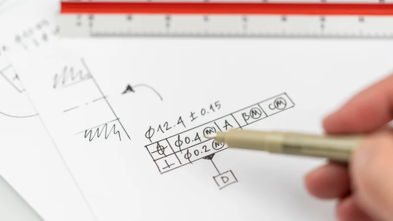
Tolerance stack up analysis looks at how dimensional variation compounds
Key Takeaways
A tolerance stack up analysis adds the dimensional variation of every part in a tolerance chain to predict the variation of one assembly-level gap or clearance.
Worst-case analysis sums tolerances arithmetically and guarantees 100% assembly, but the stack grows linearly with part count, which forces expensive tight tolerances.
The RSS method (root sum square) takes the square root of the sum of squared tolerances and predicts 99.73% conformance, typically cutting the stack by 40% to 60% on a five-part chain.
RSS is optimistic in practice because its assumptions (centered normal distribution, independence, and a tolerance equal to 3 sigma) are often violated. Inflation factors and mean shift models correct for this.
Sensitivity analysis usually shows that one or two dimensions dominate the stack, And tightening those is far cheaper than tightening everything.
Introduction
Every dimension you specify carries a tolerance, and every tolerance is a promise that the real dimension will land somewhere inside a band rather than exactly on nominal. Put five such dimensions in a line and the bands add up. Whether they add up to too great a number is what a tolerance stack up analysis answers.
A worst-case stack analysis involves addition, and an RSS stack uses Pythagoras. Both are useful, but it helps to know which assumptions each method carries.
This guide covers the basics of tolerance stack up analysis: how to build a tolerance chain, a worked five-part example in metric units, both core formulas, the inflation factors and mean shift models that keep the statistical method honest, the link to Cpk and process capability, and the point at which you should stop using a spreadsheet.
What Is a Tolerance Stack Up?

A tolerance stack up is the cumulative effect of individual tolerances on an assembly-level requirement. No process makes parts exactly at nominal, so every dimension in the chain contributes dimensional variation to the final gap, clearance, or interference you care about.
In mechanical design, that assembly requirement is often a gap that must stay positive (because parts must go together) and bounded from above (a bearing preload, a seal compression, a display flush to a bezel). Tolerance stack-up analysis is how you check both limits.
Skipping the analysis pushes the discovery of interference to first article inspection, when tooling is already cut. Running it early lets you trade tolerance against manufacturing cost while the drawing is still editable, and it tells your suppliers which dimensions genuinely need process control and which do not.
Recommended reading: Press Fit Tolerance: How to Specify Interference Fits
Building the Tolerance Chain
Before doing any tolerance stack-up calculations, first establish exactly which dimensions control the requirement and how they connect. The stack-up is a closed loop: start with the functional gap, trace through the features that locate or constrain it, and return to the other side of the gap.
Once this loop is defined, each dimension can be given a direction, converted into the form required by the calculation, and assigned an appropriate variation based on either its tolerance or actual process data.
Define the requirement: State the gap, its nominal dimension, and its performance limits (for example, “clearance between retaining ring and bearing face must stay between 0.05 mm and 0.70 mm”).
Draw the loop: Start at one side of the gap, chain dimensions head to tail through contacting features, and close the loop at the other side. Every dimension you cross belongs in the stack.
Assign signs: Dimensions that increase the gap get +1, dimensions that consume it get -1.
Convert every callout to an equal-bilateral form: A hole specified 10.0 +0.3/-0.0 becomes 10.15 ± 0.15. Bilateral tolerances around a shifted nominal are the only form the formulas accept.
Translate geometric controls: A position tolerance of Ø0.4 contributes ±0.2 to a stack.
Collect real process data: Where you have it, use measured standard deviation per dimension rather than assuming the tolerance band represents the true spread.
Skipping step 4 or step 5 is a common source of a wrong answer, and neither shows up as an obvious error in the spreadsheet.
Worked Example: A Five-Part Bearing Stack
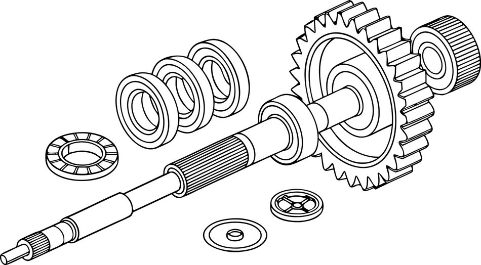
Consider a shaft assembly seated in a housing bore. The gap G is the clearance left for a retaining ring after the internal components are stacked.
Dimension | Feature | Nominal (mm) | Tolerance (mm) | Sensitivity aᵢ |
L₁ | Housing bore depth | 52.40 | ± 0.20 | +1 |
L₂ | Bearing 1 width | 15.00 | ± 0.05 | -1 |
L₃ | Spacer length | 20.00 | ± 0.10 | -1 |
L₄ | Bearing 2 width | 15.00 | ± 0.05 | -1 |
L₅ | Retaining ring thickness | 2.00 | ± 0.05 | -1 |
The nominal values give a nominal gap of 52.40 - 52.00 = 0.40 mm. Different methods of tolerance stack up analysis attempt to calculate how far the manufactured gap will or could deviate from that figure.
Sensitivity analysis
Sensitivity analysis is used to determine which individual tolerances have the biggest impact on the final assembly. In our example, the housing alone drives nearly 70% of the variation and is therefore the best candidate for tolerance tightening.
Dimension | Tolerance (mm) | Tᵢ² | Share of variance |
Housing bore depth | ± 0.20 | 0.0400 | 69.6% |
Spacer length | ± 0.10 | 0.0100 | 17.4% |
Bearing 1 width | ± 0.05 | 0.0025 | 4.3% |
Bearing 2 width | ± 0.05 | 0.0025 | 4.3% |
Retaining ring | ± 0.05 | 0.0025 | 4.3% |
Worst-Case Analysis: Arithmetic Stacking
Worst-case analysis assumes every dimension can land anywhere inside its tolerance zone, including all of them at the same extreme simultaneously. The assembly tolerance is the plain sum of the absolute contributions.[1]
T(worst case) = |a₁|T₁ + |a₂|T₂ + ... + |aₙ|Tₙ
T(worst case) = the maximum possible variation in the final gap or dimension.
Tᵢ = the tolerance of each individual dimension.
aᵢ = whether that dimension increases or decreases the result, usually +1 or −1.
|aᵢ| removes that +/− direction, because worst-case analysis assumes every dimension varies in the direction that makes the result worst.
Therefore, for a simple stack where aᵢ = ±1, you simply add all the individual tolerances together.
For the bearing stack:
T = 0.20 + 0.05 + 0.10 + 0.05 + 0.05 = 0.45 mm
So G, the gap, runs from 0.40 - 0.45 = -0.05 mm to 0.40 + 0.45 = 0.85 mm. The negative lower bound means interference is geometrically possible: some fraction of assemblies will not accept the retaining ring. The design fails worst case.
The strength of this approach is that the bound is absolute. As Scholz puts it, no matter how the detail dimensions deviate within their limits, the gap is guaranteed to stay inside the calculated range, provided your inspection process actually confirms every part is in tolerance.[1]
The weakness is that the stack grows roughly linearly with part count. If every contribution is equal, T(worst case) = n × T(detail), so the tolerance you can allow each part is the assembly tolerance divided by n. On a twenty-part chain that becomes extreme, which is why worst case is normally reserved for three or four part stacks, safety-critical interfaces, low-volume builds, and anywhere a single non-conforming assembly is unacceptable.
The RSS Method: Statistical Tolerance Analysis
The RSS method treats the deviations as random variables. Instead of adding all tolerances together, it assumes that part variations are random and follow a normal bell-curve distribution.
Statistical tolerance analysis rests on two assumptions:
Centered normal distribution: Each dimension varies according to a normal distribution centered on the middle of its tolerance interval, with the ±3 sigma spread equal to the tolerance band. (Tolerance limits are set three standard deviations above and below the average.) That places 99.73% of parts inside the limits.[1]
Independence: Each part’s deviation is statistically unrelated to the others, so positive and negative deviations partially cancel.[1]
Under those assumptions the assembly tolerance is the root sum square:
T(RSS) = √(a₁²T₁² + a₂²T₂² + ... + aₙ²Tₙ²)
For the bearing stack:
T(RSS) = √(0.20² + 0.05² + 0.10² + 0.05² + 0.05²) = √0.0575 = 0.240 mm
G now runs from 0.16 mm to 0.64 mm. The design passes, and the stack shrank by 47% against worst case.
Scholz describes the geometry behind this as a Pythagorean shortcut: for three dimensions, the worst case sum walks the three edges of a box while the RSS result cuts the diagonal. The price of the shortcut is that ±T(RSS) bounds the gap with 0.9973 probability rather than with certainty.[1]
Why RSS Is Usually Too Optimistic
Practice shows assemblies vary more than the RSS method predicts. Scholz identifies four assumptions that break down, and each has a correction.[1]
The tolerance may be tighter than reality: RSS often assumes the stated tolerance represents ±3σ, but real processes may behave closer to ±2σ. Arthur Bender’s “Benderizing” method applies a 1.5× correction to account for this, making the RSS estimate more conservative.[2]
Dimensions may not follow a bell-shaped distribution: RSS assumes normally distributed variation. Real processes can produce triangular, uniform, or other distributions. An inflation factor can be applied to each dimension to account for its actual distribution.
Processes may not be centered on nominal: A manufacturing process can consistently produce parts slightly above or below the target dimension. This mean shift does not cancel out between parts, so the shifted portions are added directly, while the remaining random variation is combined using RSS.
Dimensions may not be independent: RSS assumes each dimension varies independently. In reality, several dimensions may be affected by the same machine, tooling, temperature, or process shift, causing them to move together rather than cancel statistically.
Tolerance and Process Capability
In tolerance analysis, mean shift is the offset or drift of a manufacturing process’s average output from the nominal center target. A mean shift model connects tolerance stack-up analysis directly to process capability.[1]
Requiring that total variation stays inside the tolerance limits with a shifted mean gives:
Cpk = (1 - ηᵢ)Tᵢ / 3σᵢ ≥ 1
Cpk: measures whether the process has enough room to stay within the tolerance. This is not a stack up formula; it tells you how well a process fits inside its tolerance limits.
ηᵢ: the mean shift, expressed as a fraction of the tolerance. For example, η = 0.20 means the process average is shifted 20% away from nominal.
(1 − ηᵢ)Tᵢ: the remaining tolerance after accounting for that shift.
3σᵢ: the expected spread of the process. Dividing the remaining tolerance by 3σ tells you whether the process variation fits within the available space.
Cpk ≥ 1: means the process’s ±3σ spread fits within the tolerance limits. Cpk < 1 means some of the expected variation extends beyond the limits.
Monte Carlo Simulation and 3D Variation Analysis
RSS is a closed-form solution for a linear stack. However, it stops being adequate when the assembly function is non-linear, when tolerance zones interact in more than one direction, or when distributions differ in shape from one dimension to the next.
Monte Carlo simulation handles all three of those situations. You sample each dimension from its own distribution, evaluate the assembly function, and repeat tens of thousands of times to build an empirical distribution of the gap. The result is a predicted yield and a full histogram rather than a single ± value.
The general procedure of Monte Carlo simulation applied to tolerance analysis has three parts.[3]
Randomly generate n sets of component dimensions according to the specified distributions.
Use these dimensions to calculate the assembly function for each set.
Estimate the assembly’s performance, including its mean, standard deviation, and reject rate.
Choosing Methods and Software

Tolerance stack-up analysis can be performed at different levels of complexity, depending on how the component dimensions and geometric relationships interact. A 1D stack is appropriate for straightforward linear dimensions along a single axis, while 2D and 3D stacks are needed when angular, positional, or spatial effects become important.
The table below summarizes when each approach is appropriate and the typical methods used.
Analysis type | Use when | Typical method |
1D stack | Variation runs along a single axis through flat, parallel, contacting features | Spreadsheet, worst case and RSS method |
2D stack | Angular effects, in-plane hole patterns, or rotational play matter | Spreadsheet with sensitivity coefficients, or dedicated software |
3D stack | Datum schemes, compound angles, and geometric controls interact in space | Tolerance analysis software with Monte Carlo or system moments |
Commercial tolerance analysis software becomes increasingly useful once a stack involves 2D or 3D relationships that are difficult to represent in a spreadsheet.
Tools such as CETOL 6σ and 3DCS Variation Analyst integrate with CAD systems (including SOLIDWORKS and CATIA) to model how dimensional and geometric tolerances propagate through an assembly.[4][5] CETOL uses a Method of System Moments approach specifically to escape the RSS restrictions on distribution type and uniform quality level across 1D, 2D, and 3D analyses.[4]
These tools are particularly useful when the aim is to do more than calculate a tolerance stack. They can help identify the main sources of variation, compare alternative tolerance schemes, and estimate the likelihood that an assembly will meet its functional requirements in production.
Recommended reading: Understanding CAD File Types: A Comprehensive Guide for Digital Design and Hardware Engineers
Standards That Govern the Inputs
Your stack is only as good as the tolerances feeding it, and those come from published standards.
ASME Y14.5 (2018 edition, reaffirmed 2024) is the authoritative reference for geometric dimensioning and tolerancing in North America. It establishes the symbols, rules, definitions, and defaults for stating and interpreting GD&T on drawings and in digital data files, covering form, orientation, location, profile, and runout.[6]
ASME Y14.5.1 (2019 edition) supplies the mathematical definitions behind those symbols, including the determination of actual values, which is what makes automated tolerance stack-up calculations from a model unambiguous.[7]
ISO 286-1:2010 defines the ISO code system for tolerances on linear sizes for cylinders and pairs of parallel opposite surfaces. It is the source of the H7/g6 style callouts, and it warns that diameter tolerances alone are often insufficient to control a fit without additional form tolerances and surface texture requirements.[8]
ISO 2768-1:1989 provides general tolerances in four classes for linear and angular dimensions with no individual tolerance indication, for parts produced by metal removal or formed from sheet metal. Every unindicated dimension in your stack inherits its tolerance from here, which is exactly why an unnoticed general tolerance block can wreck a stack.[9]
Common Mistakes and How to Catch Them
Mixing worst case inputs with statistical outputs: Do not feed geometric tolerances into an RSS calculation and then quote a 99.73% yield. The inputs no longer represent a distribution.
Forgetting the general tolerance block: Unindicated dimensions still carry ISO 2768 or an equivalent standard, and they still stack.
Assuming independence across identical parts: Two bearings from the same lot share a mean shift.
Ignoring assembly-induced variation: Slippage between clearance holes and fasteners, joint compliance, and press-fit deformation are real contributors that do not appear on a part drawing.
Quoting RSS without process data: Without measured standard deviation or a Cpk figure, RSS is only an assumption.
Leaving temperature out: A 200 mm aluminum dimension moves roughly 0.1 mm over a 20 °C swing, which can exceed the entire calculated stack.
Analyzing only the minimum gap: Maximum gap failures (rattle, excessive backlash, seal under-compression) are just as real and need the other end of the range checked.
Tolerance Allocation and Manufacturing Cost
Tolerance analysis asks whether a design works, whereas tolerance allocation asks how to distribute a fixed assembly tolerance across parts at the lowest cost.
Halving a tolerance can more than double the cost of a machined part, because it moves the work to a slower process, a better machine, or a higher scrap rate.
On the other hand, strategies can be employed to both tighten tolerances and cut costs simultaneously. One group of researchers carried out a reliability-based redesign using a Jacobian-Torsor model to a three-part centering pin assembly, tightening the functional requirement from ±0.9245 mm to ±0.6318 mm while raising assembly reliability from 95.10% to 97.22% and cutting total cost by 10.93%. The gains came from reallocating tolerances across seven components rather than tightening all of them.[10]
As a general rule of thumb: run the sensitivity analysis, tighten only the top one or two contributors, and relax everything that contributes less to the stack up.
Conclusion
Tolerance stack up analysis provides several models with increasing realism and decreasing conservatism. Worst case analysis is a good starting point: if it passes, you are finished and you have a guarantee. If it fails, move to RSS, but only after you can defend the assumptions of centered normal distribution, independence, and a tolerance that represents 3 sigma.
When those assumptions are shaky, and they usually are, the mean shift model with n around 0.20 gives a defensible middle answer that most production processes can actually hold. Escalate to Monte Carlo simulation when the geometry stops being one-dimensional and you need a more thorough calculation.
Whichever method you use, the goal is to identify the tolerances that matter most, rather than simply tightening every dimension.
Frequently Asked Questions
What is the difference between tolerance analysis and tolerance allocation?
Tolerance analysis works forwards: given part tolerances, it predicts assembly variation. Tolerance allocation works backwards: given a required assembly tolerance, it distributes tolerance across parts, usually to minimize manufacturing cost. Both use the same stacking formulas, just solved in opposite directions.
How many parts before I should switch from worst case to RSS?
There is no hard rule, but worst case is most useful up to three or four contributing dimensions. Beyond that the arithmetic sum grows linearly while the RSS result grows with the square root, so the penalty for worst case becomes severe. Volume matters too: a low-volume, safety-critical assembly can justify worst case at any part count.
Why does the RSS method predict 99.73% and not 100%?
Because ±3 sigma on a normal distribution contains 99.73% of the population. The RSS result is a 3 sigma bound on the assembly variation, so it inherits that probability. The value looks arbitrary because it is the consequence of choosing the round number 3 for the sigma multiplier.
Can I use RSS if my parts are not normally distributed?
Not directly. Apply a distribution inflation factor to each contribution, for example 1.732 for a uniform distribution or 1.225 for a triangular one, or move to a Monte Carlo simulation that samples the real distributions.
How do I include GD&T controls in a 1D stack?
Convert each geometric control into an equivalent ±contribution along the direction of the stack. A diametral position tolerance of Ø0.4 contributes ±0.2. Parallelism and perpendicularity contribute their full zone width projected onto the stack direction. Where the control carries an MMC modifier, use the MMC value for worst case and model the bonus tolerance explicitly for statistical work.[11]
What Cpk should I assume if the supplier will not share data?
Assume nothing and say so. If you must proceed, Cpk = 1.0 with a mean shift fraction of 0.20 is a defensible conservative default, but flag it as an assumption in the analysis so it can be replaced once first article inspection data arrives.
Do I need software, or is a spreadsheet enough?
A spreadsheet is sufficient and preferable for 1D stacks: it is auditable, and every reviewer can follow the arithmetic. Tolerance analysis software earns its place on 2D and 3D problems where sensitivity coefficients must come from the CAD geometry rather than from your judgement.
References
[1] Scholz F. Tolerance stack analysis methods. Boeing Information and Support Services; 1995.
[2] Bender A. Statistical tolerancing as it relates to quality control and the designer (6 times 2.5 = 9). Mid-Year Meeting; 1968 May 20; Detroit, MI, USA.
[3] Yan H, Wu X, Yang J. Application of Monte Carlo method in tolerance analysis. Procedia CIRP. 2015;27:281-5.
[4] Sigmetrix. What is tolerance stack-up? Analysis methods and more [Internet]. Sigmetrix; [cited 2026 Aug 18].
[5] Metrologic DCS. 3DCS Variation Analyst: tolerance analysis software [Internet]. Montbonnot-Saint-Martin (FR): Metrologic DCS; 2026 [cited 2026 Aug 18].
[6] ASME. Y14.5 Dimensioning and tolerancing [Internet]. ASME; [cited 2026 Aug 18].
[7] ASME. Y14.5.1 Mathematical definition of dimensioning and tolerancing principles [Internet]. ASME; [cited 2026 Aug 18].
[8] ISO. ISO 286-1:2010, Geometrical product specifications (GPS): ISO code system for tolerances on linear sizes, Part 1: Basis of tolerances, deviations and fits [Internet]. Geneva: International Organization for Standardization; 2010 [cited 2026 Aug 18].
[9] ISO. ISO 2768-1:1989, General tolerances, Part 1: Tolerances for linear and angular dimensions without individual tolerance indications [Internet]. Geneva: International Organization for Standardization; 1989 [cited 2026 Aug 18].
[10] Wang B, Huang X, Chang M. Reliability-based tolerance redesign of mechanical assemblies using Jacobian-Torsor model. Sci Prog. 2021;104(2).
[11] GD&T Basics. Maximum material condition (MMC) [Internet]. GD&T Basics; [cited 2026 Aug 18].
in this article
1. Introduction2. What Is a Tolerance Stack Up?3. Building the Tolerance Chain4. Worked Example: A Five-Part Bearing Stack5. Worst-Case Analysis: Arithmetic Stacking6. The RSS Method: Statistical Tolerance Analysis7. Why RSS Is Usually Too Optimistic8. Tolerance and Process Capability9. Monte Carlo Simulation and 3D Variation Analysis10. Choosing Methods and Software11. Standards That Govern the Inputs12. Common Mistakes and How to Catch Them13. Tolerance Allocation and Manufacturing Cost14. Conclusion15. Frequently Asked Questions16. References