What is Magnetism? Examples of Magnetic Substances
Magnetism is a force exerted by charged particles in motion that allows them to attract/repel other moving charged particles. The universal phenomenon is responsible for shaping the world as we know it.

Last updated on 09 Apr, 2024. 39 minutes read

Introduction
Magnetism serves as an invisible force behind an array of everyday objects and advanced technologies alike—from the motors powering our appliances to the levitating trains redefining rapid transit, and even in the playful attraction of magnets in toys. This fundamental force is not only pivotal in the operation of generators, transformers, and audio systems but also plays a crucial role in industrial machinery, innovative furniture designs, efficient recycling devices, and much more.
At the core of our understanding are the elementary principles of magnetism: the existence of two poles, north and south, with opposite poles attracting each other and like poles repelling. Intriguingly, certain materials, notably those containing iron, naturally exhibit magnetic properties, while others like cobalt and nickel, though not magnets themselves, are drawn to magnetic fields.
This article delves into the essence of magnetism, beginning with a historical overview that traces its discovery and understanding through the ages. We explore key concepts such as Faraday’s and Lenz’s laws to grasp the underlying principles of magnetic phenomena. Furthermore, we dissect the classification, types, and properties of magnetic materials, offering illustrative examples along the way. Subsequent sections are dedicated to the principles behind electromagnets and an exploration of the Earth’s magnetosphere, shedding light on the profound impact of magnetism on our world and beyond.
History of Magnetism
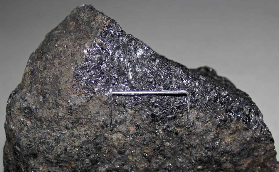
The story of magnetism begins in antiquity, with the earliest known interactions between humans and magnetic materials in Magnesia, a region in Greece. Around 600 BCE, Thales of Miletus discovered lodestones, naturally magnetized pieces of the mineral magnetite that exhibited the mysterious ability to attract iron. This natural wonder sparked interest and speculation among greeks and ancient civilizations, but it wasn't until centuries later that these forces began to be understood scientifically.
In approximately 400 BCE, Chinese scholars mentioned lodestones in their classic texts, marking the beginning of humanity's exploration into magnetism's practical applications. By the 12th century, the Chinese had innovated the use of magnetic lodestone compasses for navigation, a significant advancement that would eventually spread across the globe, revolutionizing seafaring and trade.
The scientific study of magnetism began to take shape in the 1600s with the work of William Gilbert, an English physicist who conducted systematic investigations into the behavior of magnets. Gilbert's work laid important groundwork, but it was the accidental discovery by Hans Christian Oersted in 1820 that would forever change our understanding of magnetism. Oersted observed that electric currents could influence a magnetic compass needle, a phenomenon that suggested a deep and previously unseen connection between electricity and magnetism.
This discovery led to a flurry of research and experimentation. Notable scientists such as Andre Marie Ampere, Michael Faraday, and James Clerk Maxwell made critical contributions, with Maxwell's equations eventually unifying the concepts of electricity and magnetism into a single theory of electromagnetism. While Maxwell's work encompassed a broader range of phenomena, including electromagnetic waves, the focus here remains on magnetism and its intrinsic relationship with electric currents.
In the centuries that followed, the study of magnetism continued to evolve, with advancements in understanding brought about by the development of quantum mechanics and quantum electrodynamics. Scientists like Werner Heisenberg further refined our comprehension of magnetism at the quantum level, revealing the complex and fascinating nature of magnetic forces.[1]
The journey from ancient lodestones to quantum electrodynamics illustrates humanity's enduring fascination with magnetism. It's a story of gradual discovery, where ancient observations led to scientific inquiry, and where inquiry led to a deepened understanding of the natural world. This narrative highlights the pivotal role of magnetism in the development of navigation, communication, and beyond, underscoring its importance in both historical and modern contexts.
What is Magnetism?
Magnetism emerges from the movement of electric charges or the inherent properties of specific materials, enabling them to generate forces that attract or repel other objects. This phenomenon is rooted in the intrinsic characteristics of subatomic particles, such as electrons, which, besides having mass and charge, possess something known as an intrinsic magnetic moment, contributing to their magnetic properties.
Laws of Magnetism
To grasp the origins of magnetism, it's pivotal to understand electromagnetic induction, illuminated by two foundational principles:
Faraday's Law: Faraday's Law articulates that an electromotive force (emf) is induced in a conductor when it is exposed to a changing magnetic field. This law reveals how electricity can be generated from magnetic fields, a principle at the heart of many electrical devices and systems.
Lenz's Law: Lenz's Law further specifies that the induced emf always acts to oppose the change in the magnetic field that produced it. This opposition is a manifestation of energy conservation, ensuring that the induced magnetic field counteracts the original field's changes.
Magnetic Fields: Magnetic fields, generated by moving electric charges or changing electric fields, are regions in space where magnetic lines of forces can be detected. The direction of a magnetic field is represented by magnetic field lines, with the strength determined by the density of these lines. The SI unit for magnetic field strength is the tesla (T).
Magnetic field strength is a measure of the force exerted per ampere per meter on a current-carrying conductor within a magnetic field. Given the Tesla's magnitude, the Gauss (G) is often used for more practical measurements. For context, Earth's magnetic field strength is approximately 0.0000305 T, or 0.3 G, illustrating the subtle yet essential influence of magnetism on our planet and beyond.
Magnetic flux (Φ): Magnetic flux, a measure of the total magnetic field passing through an area, is defined as the product of the magnetic flux density (B) and the area (A) perpendicular to the field lines:
Φ = B · A
where B is in teslas (T) and A is in square meters (m²).
Lorentz law: The Lorentz force law describes the relationship between magnetic fields and forces. A moving electric charge (q) with velocity (v) in a magnetic field (B) experiences a force (F) given by:
F = q(v × B)
The force is perpendicular to both the velocity and the magnetic field, following the right-hand rule.
Current-carrying conductors also experience forces in magnetic fields. The force (F) on a wire with current (I), length (L), and angle (θ) between the current and the magnetic field (B) is:
F = ILB sin(θ)
This relationship is crucial for the operation of electromagnetic devices, such as motors and generators.
Biot-Savart law: The magnetic field at a point due to a current-carrying wire can be calculated using the Biot-Savart law:
dB = (μ₀I / 4π) · (dl × r̂) / r²
where dB is the differential magnetic field, μ₀ is the permeability of free space, I is the current, dl is the differential length element, r̂ is the unit vector pointing from the wire to the point, and r is the distance between them.
Ampere's circuital law: Ampere's circuital law relates the magnetic field around a closed loop to the current passing through it:
∮ B · dl = μ₀I
where ∮ denotes the line integral around the closed loop, and I is the total current enclosed by the loop.
These laws, along with Maxwell's equations, provide a comprehensive framework for understanding and analyzing magnetic fields and forces in various applications, from electromagnetic devices to particle accelerators and magnetic resonance imaging (MRI) systems.
Magnetic Poles and Dipoles
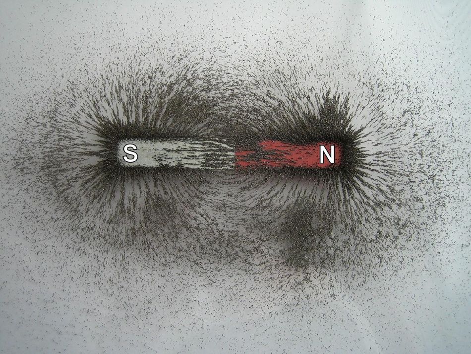
Magnetic poles, located at the ends of a magnet, are regions where the magnetic field is strongest. There are two types of poles: north and south. Opposite poles attract, while like poles repel. This behavior is similar to electric charges.
A magnetic dipole is a pair of equal and opposite magnetic poles separated by a small distance. Dipoles are the fundamental building blocks of magnetic systems. The magnetic field generated by a dipole is characterized by field lines that form closed loops, originating from the north pole and terminating at the south pole.
The magnetic scalar potential (Φ) at a point (r, θ) due to a dipole with magnetic moment (m) is given by:
Φ(r, θ) = (μ₀m / 4πr²) · cos(θ)
where μ₀ is the permeability of free space, r is the distance from the dipole, and θ is the angle between the dipole moment and the position vector.
The magnetic field (B) can be obtained from the magnetic scalar potential using the gradient operator:
B = -∇Φ
Alternatively, the magnetic vector potential (A) can be used to calculate the magnetic field:
B = ∇ × A
The magnetic vector potential due to a dipole with magnetic moment (m) at a point (r) is given by:
A(r) = (μ₀m / 4πr²) × r̂
where r̂ is the unit vector pointing from the dipole to the point.
The force between two magnetic dipoles with moments m₁ and m₂, separated by a displacement vector r, is given by:
F = (3μ₀ / 4πr⁵) · [r · (m₁ · m₂) + m₁ · (r · m₂) + m₂ · (r · m₁) - 5(r · m₁)(r · m₂) / r²]
This equation demonstrates the complex nature of dipole-dipole interactions, which depend on the relative orientation and separation of the dipoles.
Magnetic effects of atoms and subatomic particles
The magnetic properties of atoms and subatomic particles, particularly electrons, are critical in understanding magnetism on a microscopic scale. Electrons orbiting an atom, while simultaneously exhibiting electron spins on their own axes, effectively function as tiny current loops, generating magnetic fields. This phenomenon leads to the principle that electrically charged particles inherently possess magnetic properties.
However, the contribution of these so-called orbital magnetic fields to an atom's overall magnetic behavior is not straightforward. In atoms where electron shells are completely filled, electrons pair up, each spinning in opposite directions. This arrangement results in the cancellation of their magnetic effects, leading to a net magnetic field of zero.
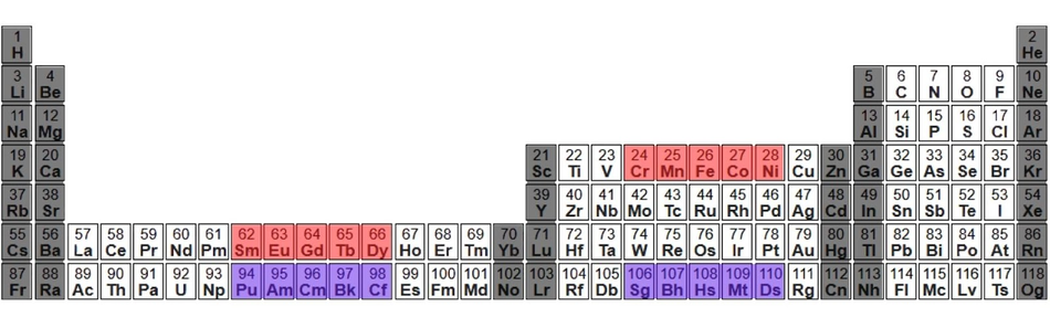
The magnetic nature of an atom largely depends on its electron configuration, particularly in the context of the periodic table. Atoms with full or nearly full outer shells, typically found at the edges of the s/p/d blocks, exhibit no magnetic properties due to this cancellation effect. Conversely, elements positioned in the middle of these blocks—such as manganese, iron, cobalt, and nickel—have unpaired electrons in their outer shells, making them inherently magnetic. These elements are also among the most common magnetic metals.
When atoms come together to form a crystalline structure, they have the potential to align their magnetic fields either in the same direction or in opposite ones. In nature, atoms tend toward configurations that minimize energy. Therefore, the collective magnetic orientation of atoms within a material can significantly influence its magnetic properties. For instance, chromium, despite having atoms with strong magnetic properties, forms a material that is not magnetically ordered due to the antiparallel alignment of its internal magnetic fields. This alignment contrasts with the collective behavior seen in ferromagnetic materials, where magnetic fields align to produce a strong external magnetic effect.
Types of Magnetic Materials
The magnetic properties of materials are deeply influenced by the arrangement and behavior of electrons within atoms. Electrons in motion, akin to tiny current loops, generate magnetic moments. When electrons pair up, their opposite spins result in the cancellation of these moments, leaving no net magnetic effect. However, unpaired electrons contribute to a net magnetic moment, imparting magnetic properties to the atom.
Considering this, one might ponder the effect of bringing a magnet close to an atom characterized entirely by paired electrons. Intuitively, it might seem such an atom would remain unaffected, neither attracted nor repelled by the magnet due to the absence of a net magnetic moment. Yet, this assumption misses a crucial aspect of magnetic interactions: electromagnetic induction.
Electromagnetic induction introduces a dynamic layer to the interaction between magnetic fields and materials. Even in the presence of solely paired electrons, an external magnetic field can induce subtle electromagnetic effects within the material, showcasing the nuanced and complex nature of magnetic interactions beyond mere attraction and repulsion. This principle underscores the intricate relationship between magnetic fields and material properties, extending the scope of magnetic influence to a broader array of materials and conditions.
The Langevin function describes the magnetization of paramagnetic materials:
M = M_s * (coth(μH/kT) - kT/μH)
where M_s is the saturation magnetization, μ is the magnetic moment of an atom, k is the Boltzmann constant, and T is the temperature.
The Brillouin function describes the magnetization of ferromagnetic materials:
M = M_s * (2J + 1)/2J * coth((2J + 1)μH/2JkT) - 1/2J * coth(μH/2JkT)
where J is the total angular momentum quantum number.
These functions provide a quantum mechanical description of the magnetic behavior of materials, taking into account the discrete nature of atomic magnetic moments and their response to thermal energy and external fields.
Diamagnetic Materials
When a magnet approaches an atom that possesses only paired electrons, an intriguing dynamic unfolds: the magnetic field of one electron's current loop is enhanced, while that of its counterpart—spinning in the opposite direction—is weakened. This disruption prevents the currents from neutralizing each other as they normally would.
The magnet then simultaneously attracts one electron and repels the other, but the force of repulsion predominates. This imbalance gently nudges the atom to repel the approaching magnet. Consequently, this interaction gives birth to a faint magnetic moment in opposition to the magnet, manifesting the phenomenon known as diamagnetism.
Susceptibility: Magnetic susceptibility (χ), a dimensionless measure, characterizes the response of a material to an external magnetic field. It is defined as the ratio of the induced magnetization (M) to the applied magnetic field (H):
χ = M / H
It reflects the relationship between the applied magnetic field and the resultant magnetic field within the material, influenced by its inherent properties and external conditions. In diamagnetic materials, this susceptibility is notably small and negative, indicating that the internal magnetic field developed is in opposition to the external field, revealing the material's inherent tendency to repel the magnetic influence.
Diamagnetic Materials materials are characterized by their gentle repulsion from magnetic fields. Upon encountering an external magnetic influence, diamagnetic substances instinctively generate a slight magnetic field that opposes the direction of the applied field, leading to their repulsion.
This reaction is fleeting; the moment the external field is withdrawn, the electrons' paired arrangements neutralize any induced magnetic moments, causing the material to relinquish its magnetized state. Thus, the phenomenon of diamagnetism is inherently temporary, manifesting only in the presence of an external magnetic force.
Examples of diamagnetic materials include Bismuth, Water, Copper, Diamond, Gold, Lead, Mercury, Hydrogen, Nitrogen, Silver, Silicon, Phosphorus, Antimony, and more.
Properties of Diamagnetic Materials
Exhibit weak repulsion from magnetic fields.
Tend to orient perpendicularly to the applied magnetic field.
Diamagnetic behavior is unaffected by temperature changes.
Any material with paired electrons possesses a level of diamagnetism.
Paramagnetic Materials
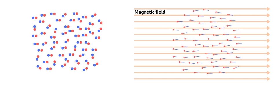
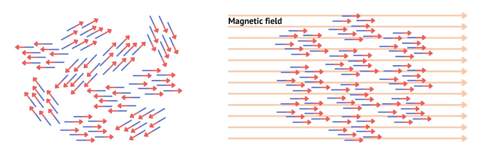
Building on the previous insights, we shift focus to materials composed of atoms with unpaired electrons. These atoms each possess a distinct magnetic moment, resulting from the unpaired electron's current loop. In the absence of an external magnetic field, these moments are randomly oriented, effectively neutralizing one another and resulting in no overall magnetization.
Upon introducing such a material to a magnetic field, say from a bar magnet, the situation changes. The atomic dipoles adjust their orientation to align with the magnetic field, albeit imperfectly due to the material's thermal energy. This misalignment means the material is only weakly attracted to the magnet, and its magnetization remains moderate. Moreover, as temperature rises, thermal agitation increases, further disrupting the alignment and diminishing the magnetization.
Paramagnetic materials exhibit a small and positive magnetic susceptibility, indicating their tendency to be weakly attracted to magnetic fields.
Paramagnetic materials align with the external field, creating a magnetic response in the same direction, which leads to their attraction. However, this magnetization is not permanent; once the external field is removed, the atomic magnetic moments revert to their initial, disordered state, erasing the magnetization.
It's important to note that the presence of unpaired electrons doesn't guarantee paramagnetism. In fact, diamagnetism is more widespread, with most elements displaying it due to their electrons' paired configurations. Paramagnetism becomes prominent only in materials where the effect of unpaired electrons overpowers the inherent diamagnetism. Interestingly, in some elements with unpaired electrons, like copper, silver, and gold, diamagnetic behavior prevails, causing them to be repelled by magnetic fields.
Examples of paramagnetic materials include Oxygen, Calcium, Aluminum, Chromium, Lithium, Magnesium, Platinum, Tungsten, Niobium, Samarium (at room temperature), and more.
The quantum mechanical description of paramagnetism involves the Langevin function, which describes the average magnetization of a paramagnetic material:
M = M_s * (coth(μH/kT) - kT/μH)
where M is the magnetization, M_s is the saturation magnetization, μ is the magnetic moment of an atom, H is the applied magnetic field, k is the Boltzmann constant, and T is the temperature.
For paramagnetic materials with quantized angular momentum, the Brillouin function is used:
M = M_s * (2J + 1)/2J * coth((2J + 1)μH/2JkT) - 1/2J * coth(μH/2JkT)
where J is the total angular momentum quantum number.
The Van Vleck equation provides a more general description of the magnetic susceptibility, taking into account the contributions from both paramagnetic and diamagnetic terms:
χ = (N/V) * (μ_0μ_B2/3kT) * Σ_n (E_n - E_0) * |⟨n|L+2S|0⟩|2 * exp(-(E_n-E_0)/kT)
where N is the number of atoms, V is the volume, μ_B is the Bohr magneton, E_n and E_0 are the energies of the excited and ground states, respectively, and ⟨n|L+2S|0⟩ is the matrix element of the angular momentum operator between the ground and excited states.
These equations provide a more accurate description of the magnetic behavior of paramagnetic and diamagnetic materials, considering the discrete nature of atomic magnetic moments and their response to thermal energy and external fields.
Properties of Paramagnetic Materials
Weakly attracted to magnetic fields.
Attempt to align with the direction of an applied magnetic field.
Attraction diminishes with rising temperature.
Exhibited by elements with unpaired electrons and minimal diamagnetic influence.
Ferromagnetic materials
While most elements, including those with unpaired electrons, show no significant magnetic attraction or repulsion, four unique elements in the periodic table stand out for their strong attraction to magnets. This distinction arises not just from their unpaired electrons but from differences in their crystal structures compared to paramagnetic materials.
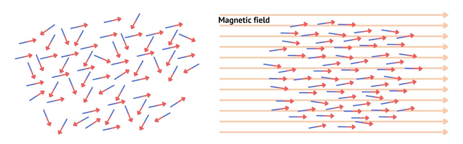
Ferromagnetic materials are characterized by the presence of magnetic domains—groups of atoms whose magnetic moments point in the same direction. When exposed to a magnetic field, these domains realign, collectively orienting in the direction of the field, thereby creating a unified, strongly magnetized domain. This interaction leads to the material exhibiting extremely strong magnetization.
In the presence of a magnetic field, ferromagnetic materials develop a significant magnetic moment that aligns with the field, drawing the material towards the magnet. The intensity of this magnetization continues to increase until reaching a saturation point, beyond which additional increases in the external magnetic field have no further effect on magnetization.
The response of ferromagnetic materials to the removal of the external magnetic field is determined by their retentivity—the ability to retain magnetization post-exposure.
Soft ferromagnetic materials tend to lose their magnetization quickly, making them ideal for applications requiring temporary magnetization, such as in electrical machine cores. In contrast, hard ferromagnetic materials maintain their magnetization, serving as the basis for creating permanent magnets due to their high coercivity, or resistance to demagnetization.
Examples of ferromagnetic materials include Iron, Cobalt, Nickel, and Gadolinium.
Ferromagnetic materials form magnetic domains, regions where the atomic magnetic moments align in the same direction, separated by domain walls. The formation of domains minimizes the overall magnetic energy of the system by reducing stray magnetic fields outside the material. The domain structure can be observed using techniques such as magnetic force microscopy (MFM) and Lorentz transmission electron microscopy (LTEM).
The magnetic behavior of ferromagnetic materials is described by the hysteresis loop, which plots the induced magnetization (M) as a function of the applied magnetic field (H). Key parameters of the hysteresis loop include:
Saturation magnetization (M_s): The maximum magnetization achieved when all magnetic moments align with the applied field.
Remanence (M_r): The remaining magnetization when the applied field is reduced to zero after reaching saturation.
Coercivity (H_c): The reverse magnetic field required to reduce the magnetization to zero after reaching saturation.
The shape and size of the hysteresis loop depend on the material's composition, microstructure, and temperature. Hard magnetic materials (high coercivity) are used for permanent magnets, while soft magnetic materials (low coercivity) are used in transformers and electromagnets.
The magnetization process in ferromagnetic materials is described by the Brillouin function:
M = M_s * (2J + 1)/2J * coth((2J + 1)μH/2JkT) - 1/2J * coth(μH/2JkT)
where M_s is the saturation magnetization, J is the total angular momentum quantum number, μ is the magnetic moment of an atom, k is the Boltzmann constant, and T is the temperature.
Above the Curie temperature (T_C), the thermal energy overcomes the exchange interaction, and the material becomes paramagnetic. The magnetic susceptibility (χ) of ferromagnetic materials above T_C is described by the Curie-Weiss law:
χ = C / (T - T_C)
where C is the Curie constant.
The temperature dependence of the saturation magnetization can be approximated by the Bloch law:
M_s(T) = M_s(0) * (1 - (T/T_C)(3/2))
where M_s(0) is the saturation magnetization at absolute zero.
The exchange interaction between neighboring magnetic moments can be described by the Heisenberg Hamiltonian:
H = -Σ J_ij * S_i · S_j
where J_ij is the exchange integral between moments S_i and S_j.
These equations provide a quantitative framework for understanding the magnetic properties of ferromagnetic materials and their dependence on temperature and atomic-scale interactions.
Properties of Ferromagnetic Materials
Strongly attracted to and aligned with magnetic fields.
Ferromagnetism decreases with temperature increase.
Above Curie temperature, they turn paramagnetic.
Presence of unpaired electrons and magnetic domains.
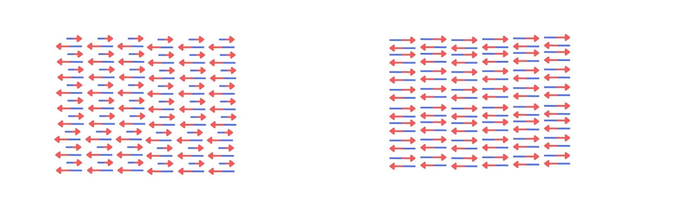
Antiferromagnetism and Ferrimagnetism
When adjacent magnetic moments in a material align in opposite directions (antiparallel), the material exhibits antiferromagnetism, where the opposing magnetic moments cancel out, resulting in no net magnetism. In contrast, ferrites or ferrimagnetic materials also feature antiparallel magnetic moments, but with varying magnitudes, leading to a net magnetization in the material.
Examples of antiferromagnetic materials include Manganese Oxide, Manganese Sulfide, Chromium Oxide, Nichrome, and more.
Examples of ferrimagnetic substances include metal oxides like magnetite.
Ferromagnetic materials have large, positive susceptibilities (102 to 106), paramagnetic materials have small, positive susceptibilities (10-3 to 10-5), and diamagnetic materials have small, negative susceptibilities (around -10-5).
The magnetization curve, plotting induced magnetization (M) vs. applied magnetic field (H), provides valuable insights into a material's magnetic properties. Ferromagnetic materials exhibit a nonlinear magnetization curve with hysteresis, while paramagnetic and diamagnetic materials have linear magnetization curves without hysteresis.
Types of Magnets
Based on the duration of magnetic effects, magnets are classified into the following categories:
Permanent Magnets
Materials that retain their magnetic properties for a long period of time are called permanent magnets. Ferromagnetic materials, including iron, nickel, cobalt, and some rare earth metals alloys like the ones that use Neodymium are used to make permanent magnets.
AlNiCo magnets are made up of aluminum, nickel, and cobalt and remain one of the most widely used permanent magnets. They are not as strong as magnets made with rare-earth elements but are more readily available.
Temporary Magnets
Materials that simply act as magnets under the influence of a magnetic field, and lose their magnetic properties as soon as the external field is removed, are called temporary magnets. Any current carrying conductor can behave as a temporary magnet.
Electromagnets
Electricity and magnetism are just like the two sides of the same coin, much like how Mass-Energy and Time-Space are.
When an electric current is made to flow through a conductor, a magnetic field is set up around it, the direction of which can be determined by the right-hand thumb rule. This effect is intensified by wrapping a wire over a soft ferromagnetic core and the resulting setup becomes an electromagnet.

Electromagnets are among the most popular temporary magnets used in a number of applications, including electric motors, radios, and several other household devices and industrial systems. The strength of the electromagnet can be accurately adjusted by changing the number of turns of the electromagnet coil, the dimensions of the electromagnet, or the core material.
Earth’s magnetic field
The source or causes of the earth’s magnetic field are not completely understood yet. However, it is believed that the earth’s magnetism is due to its metal core. The outer core contains liquid metal, and the inner core is under such a high pressure that the metal solidifies.
There is a continuous flow of electricity in the earth’s core which sets up a magnetic field around the planet. The earth, as a whole, behaves as a giant bar magnet. The magnetic field at the poles points vertically up/down at the north-south poles of the planet. The earth's magnetic poles lie slightly away from geographic poles and gradually keep changing their position over time.
Earth’s magnetosphere shields the planet from the solar wind. The solar wind is composed of streaming charged particles like protons and electrons from the sun. Some of these particles have high radiation energies that can cause damage to life on earth. But the presence of the earth’s magnetic field deflects most of the particles in the solar wind to protect the planet.
A compilation of beautiful aurora lights as visible from some Nordic countries.
When the solar wind comes in contact with the earth’s magnetosphere, it creates a magnetic storm that stretches the magnetosphere while bringing some charged particles towards the earth. When these particles come in contact with neutral oxygen and nitrogen atoms in the atmosphere, they emit light. This phenomenon gives rise to the aurora borealis or aurora australis (northern/southern lights).
Without the earth’s magnetosphere, the earth’s atmosphere and life as we know it wouldn’t exist.
Applications of Magnetism in Engineering
Magnetism plays a crucial role in numerous engineering and technological applications, enabling the development of efficient, reliable, and innovative devices and systems. From power generation and conversion to sensing and data storage, the unique properties of magnetic materials are exploited to achieve desired functionalities and performance characteristics.
Electrical machines, such as motors and generators, rely on the interaction between magnetic fields and electric currents to convert electrical energy into mechanical energy, or vice versa. In electric motors, the magnetic field generated by the stator interacts with the magnetic field produced by the rotor, resulting in a torque that causes the rotor to rotate. The efficiency and performance of electric motors depend on factors such as the strength and distribution of the magnetic fields, the properties of the magnetic materials used, and the design of the rotor and stator geometry.
Permanent magnet synchronous motors (PMSMs) utilize high-performance rare-earth magnets, such as neodymium-iron-boron (NdFeB) or samarium-cobalt (SmCo), to create a strong, stable magnetic field in the rotor. The interaction between this field and the rotating magnetic field produced by the stator windings results in high torque density and efficiency. The design of PMSMs involves optimizing the magnet shape, placement, and orientation to achieve the desired motor characteristics, such as high power density, wide speed range, and low cogging torque.
The torque (T) produced by a PMSM can be expressed as:
T = (3/2) * p * [λ_m * I_q + (L_d - L_q) * I_d * I_q]
where p is the number of pole pairs, λ_m is the permanent magnet flux linkage, I_d and I_q are the direct and quadrature axis currents, and L_d and L_q are the direct and quadrature axis inductances.
Magnetic sensors, such as Hall effect sensors and magnetoresistive sensors, exploit the change in magnetic properties or the interaction between magnetic fields to provide accurate and reliable measurements of various physical quantities, such as position, speed, and current.
Hall effect sensors measure the voltage (V_H) generated perpendicular to an electric current (I) in the presence of a magnetic field (B), given by:
V_H = (R_H * I * B) / t
where R_H is the Hall coefficient and t is the thickness of the Hall element.
Magnetoresistive sensors, including anisotropic magnetoresistance (AMR) and giant magnetoresistance (GMR) sensors, rely on the change in electrical resistance of a magnetic material in response to an external magnetic field. AMR sensors exhibit a change in resistance (ΔR) depending on the angle (θ) between the current flow and the magnetization direction, described by:
ΔR/R = (ΔR/R)_max * cos2(θ)
where (ΔR/R)_max is the maximum resistance change.
GMR sensors, comprising alternating layers of ferromagnetic and non-magnetic materials, show a significant change in resistance when exposed to a magnetic field, with the resistance change given by:
ΔR/R = (ΔR/R)_max * (1 - cos(θ)) / 2
where θ is the angle between the magnetizations of the ferromagnetic layers.
Data storage devices, such as hard disk drives (HDDs) and magnetic tape systems, rely on magnetism to store and retrieve information. In HDDs, data is stored in the form of magnetic domains on a thin magnetic coating deposited on a rotating disk. The read/write head generates a localized magnetic field to write data by selectively magnetizing the domains and senses the magnetic field variations caused by the magnetized domains to read the stored data.
Perpendicular magnetic recording (PMR) technology, which aligns the magnetic domains vertically rather than horizontally, has enabled higher storage densities compared to conventional longitudinal recording. The use of high-anisotropy magnetic materials, such as L10-ordered FePt alloys, and advanced head designs, like the tunneling magnetoresistive (TMR) head, have further pushed the boundaries of HDD capacity and performance.
The areal density (AD) of a PMR HDD can be expressed as:
AD = (N_t * N_b) / (W_t * W_b)
where N_t and N_b are the number of tracks per inch and bits per inch, respectively, and W_t and W_b are the track width and bit length, respectively.
The design and optimization of magnetic components and systems in engineering applications require a deep understanding of the underlying magnetic principles, material properties, and device physics. Engineers use advanced simulation tools, such as finite element analysis (FEA) and micromagnetic modeling, to predict the behavior of magnetic devices and optimize their performance. These tools solve the governing equations, such as Maxwell's equations and the Landau-Lifshitz-Gilbert (LLG) equation, to calculate the magnetic field distribution, magnetization dynamics, and device characteristics.
The LLG equation, which describes the precessional motion and damping of the magnetization (M) in a ferromagnetic material, is given by:
dM/dt = -γ * (M × H_eff) + (α/M_s) * (M × dM/dt)
where γ is the gyromagnetic ratio, H_eff is the effective magnetic field, α is the damping constant, and M_s is the saturation magnetization.
By leveraging the unique properties of magnetic materials and the principles of electromagnetism, engineers can design and develop efficient, reliable, and innovative devices and systems that meet the ever-increasing demands of modern technology. As the understanding of magnetic phenomena continues to advance, along with the development of new magnetic materials and manufacturing techniques, the potential for novel and transformative applications of magnetism in engineering is boundless.
Electrical Machines and Transformers
Electrical machines and transformers are essential components in power generation, transmission, and distribution systems, as well as in various industrial applications. These devices rely on the principles of magnetism to convert energy between electrical and mechanical forms or to transfer electrical energy between circuits at different voltage levels.
Electric motors and generators utilize the interaction between magnetic fields and electric currents to perform energy conversion. In an electric motor, electrical energy is converted into mechanical energy, while in a generator, mechanical energy is converted into electrical energy.
The working principle of electric motors is based on the Lorentz force, which states that a current-carrying conductor placed in a magnetic field experiences a force. In a typical DC motor, a rotating armature (rotor) is placed between permanent magnets (stator), creating a magnetic field. When a current is passed through the armature windings, a magnetic field is generated around the conductors, interacting with the stator's magnetic field. This interaction produces a torque that causes the armature to rotate.
The torque (τ) produced by a DC motor can be expressed as:
τ = K_T * I_a
where K_T is the torque constant and I_a is the armature current.
In an AC motor, such as an induction motor, the stator windings are energized with a polyphase AC supply, creating a rotating magnetic field. This rotating field induces currents in the rotor windings or bars, which in turn generate a magnetic field that interacts with the stator field, producing torque and causing the rotor to rotate.
The synchronous speed (n_s) of an AC motor is given by:
n_s = (120 * f) / p
where f is the frequency of the AC supply and p is the number of poles.
Generators convert mechanical energy into electrical energy through the principle of electromagnetic induction. When a conductor moves in a magnetic field, an electromotive force (EMF) is induced in the conductor. In a generator, the rotor is mechanically driven by an external prime mover, such as a turbine, causing the rotor windings to move through the magnetic field produced by the stator. This motion induces an EMF in the rotor windings, which is then rectified and supplied to the load.
The induced EMF (E) in a generator can be calculated using Faraday's law:
E = -N * (dΦ/dt)
where N is the number of turns in the winding and dΦ/dt is the rate of change of magnetic flux.
Transformers are static electrical devices that transfer energy between circuits at different voltage levels through the principle of electromagnetic induction. A transformer consists of two or more windings (primary and secondary) wound around a common magnetic core. When an alternating current is passed through the primary winding, it creates a time-varying magnetic flux in the core. This flux induces an EMF in the secondary winding, which is proportional to the ratio of the number of turns in the primary and secondary windings.
The voltage transformation ratio (a) of a transformer is given by:
a = N_p / N_s = V_p / V_s
where N_p and N_s are the number of turns in the primary and secondary windings, respectively, and V_p and V_s are the primary and secondary voltages, respectively.
The efficiency (η) of a transformer can be calculated as:
η = (P_out / P_in) * 100%
where P_out is the output power delivered to the load and P_in is the input power supplied to the transformer.
Transformers play a crucial role in power systems by enabling the efficient transmission of electrical energy over long distances. By stepping up the voltage at the generation site and stepping it down at the distribution level, transformers help minimize power losses and improve the overall efficiency of the power system.
The design and operation of electrical machines and transformers involve various factors, such as the choice of magnetic materials, winding configurations, insulation systems, and cooling methods. Engineers use advanced computational tools, such as finite element analysis (FEA), to optimize the performance, efficiency, and reliability of these devices.
For example, in the design of a high-efficiency transformer, engineers may use grain-oriented silicon steel for the core material to minimize hysteresis and eddy current losses. They may also employ advanced winding techniques, such as foil windings or litz wire, to reduce skin effect and proximity effect losses in the conductors.
The equivalent circuit model of a transformer can be used to analyze its performance and calculate various parameters, such as the voltage regulation (VR) and the power losses. The equivalent circuit consists of the primary and secondary winding resistances (R_p and R_s), the leakage inductances (X_p and X_s), the magnetizing inductance (X_m), and the core loss resistance (R_c).
The voltage regulation of a transformer can be calculated as:
VR = (V_s_nl - V_s_fl) / V_s_fl * 100%
where V_s_nl is the no-load secondary voltage and V_s_fl is the full-load secondary voltage.
In the case of electric motors, the use of permanent magnets, such as neodymium-iron-boron (NdFeB) or samarium-cobalt (SmCo), can significantly improve the power density and efficiency compared to conventional induction motors. The design of the rotor and stator geometry, along with the optimization of the air gap and the winding configuration, can further enhance the motor's performance and reduce cogging torque and torque ripple.
The advancement of power electronics and control systems has also revolutionized the field of electrical machines and transformers. Variable frequency drives (VFDs) and solid-state transformers (SSTs) are examples of modern technologies that offer improved efficiency, controllability, and flexibility in the operation of these devices.
VFDs allow for the precise control of motor speed and torque by varying the frequency and voltage of the AC supply. This enables energy savings, smooth operation, and extended motor life in various applications, such as pumps, fans, and compressors.
SSTs, on the other hand, are power electronic devices that combine the functions of a transformer, power converter, and control system in a single unit. They offer several advantages over traditional transformers, such as voltage regulation, power quality improvement, and the ability to interface with renewable energy sources and energy storage systems.
The modular multilevel converter (MMC) topology is a popular choice for SSTs due to its scalability, redundancy, and ability to generate high-quality output waveforms. The MMC consists of multiple submodules connected in series, each containing a capacitor and a pair of switching devices. By controlling the switching of the submodules, the MMC can generate a stepped output voltage waveform that closely approximates a sinusoidal waveform, reducing harmonic distortion and improving power quality.
The design and control of MMC-based SSTs involve various challenges, such as capacitor voltage balancing, circulating current suppression, and fault tolerance. Advanced control strategies, such as model predictive control (MPC) and sliding mode control (SMC), have been proposed to address these challenges and optimize the performance of SSTs.
In addition to the technical aspects, the development of electrical machines and transformers also considers environmental and sustainability factors. The use of eco-friendly materials, such as biodegradable insulation systems and recycled copper, along with the design for recyclability and lifecycle assessment, are becoming increasingly important in the industry.
Furthermore, the integration of electrical machines and transformers with renewable energy sources, such as wind and solar power, presents new opportunities and challenges. The variable and intermittent nature of renewable energy requires innovative solutions, such as the use of doubly-fed induction generators (DFIGs) in wind turbines and the development of smart transformers that can adapt to the changing grid conditions.
The DFIG consists of a wound rotor induction machine with the stator directly connected to the grid and the rotor connected to the grid through a partially rated power converter. This configuration allows for variable-speed operation and improved energy capture in wind turbines. The power converter controls the rotor current to optimize the generator's performance and provide reactive power support to the grid.
Smart transformers, equipped with advanced sensors, communication systems, and control algorithms, can dynamically adjust their operating parameters to maintain stable grid operation in the presence of renewable energy sources. They can also provide ancillary services, such as voltage regulation, harmonic mitigation, and fault current limitation, enhancing the overall stability and reliability of the power system.
Further Reading: Stepper vs Servo Motors: What's the Difference?
As the world moves towards a more sustainable and decarbonized energy future, the role of electrical machines and transformers in enabling the integration of renewable energy and supporting the development of smart grids will become increasingly critical. The continued research and innovation in this field will be essential to address the challenges and seize the opportunities presented by the energy transition.
Magnetic Sensors and Actuators
Magnetic sensors and actuators are essential components in various engineering applications, enabling the detection, measurement, and control of physical quantities based on magnetic principles. These devices exploit the interaction between magnetic fields and materials to provide accurate and reliable sensing and actuation capabilities.
Magnetic sensors, such as Hall effect sensors and magnetoresistive sensors, detect and measure magnetic fields or the presence of ferromagnetic objects. They convert magnetic field variations into electrical signals, which can be processed and interpreted by electronic circuits.
Hall effect sensors are based on the Hall effect, which states that when a current-carrying conductor is placed in a magnetic field perpendicular to the current flow, a voltage is generated perpendicular to both the current and the magnetic field. The generated Hall voltage (V_H) is proportional to the applied magnetic field (B), the current (I), and the inverse of the conductor thickness (t):
V_H = (R_H * I * B) / t
where R_H is the Hall coefficient, which depends on the material properties.
Hall effect sensors find applications in position sensing, speed detection, and current measurement. For example, in brushless DC motors, they detect the rotor magnet position and provide feedback for commutation. In current sensing, they measure the magnetic field generated by the current flowing through a conductor, enabling non-intrusive and isolated measurement.
Magnetoresistive sensors, such as anisotropic magnetoresistance (AMR) and giant magnetoresistance (GMR) sensors, rely on the change in electrical resistance of a magnetic material in response to an external magnetic field. AMR sensors consist of a thin strip of ferromagnetic material, typically permalloy (NiFe), whose resistance varies with the angle (θ) between the current flow and the magnetization direction:
ΔR/R = (ΔR/R)_max * cos2(θ)
where (ΔR/R)_max is the maximum resistance change.
AMR sensors are used in compass navigation, rotary encoders, and current sensing, offering high sensitivity, low noise, and a wide operating temperature range.
GMR sensors consist of alternating layers of ferromagnetic and non-magnetic materials, exhibiting a significant resistance change when exposed to a magnetic field:
ΔR/R = (ΔR/R)_max * (1 - cos(θ)) / 2
where θ is the angle between the magnetizations of the ferromagnetic layers.
GMR sensors find applications in high-density data storage, magnetic field sensing, and biosensing, offering higher sensitivity and a larger resistance change compared to AMR sensors.
Magnetic actuators, such as solenoids and relays, convert electrical energy into mechanical motion using magnetic principles. Solenoids consist of a coil wound around a movable ferromagnetic core (armature). When current passes through the coil, a magnetic field is generated, attracting the armature. The force (F) generated by a solenoid is proportional to the square of the current (I) and the number of turns (N) in the coil:
F = (μ_0 * N2 * I2 * A) / (2 * g2)
where μ_0 is the permeability of free space, A is the coil cross-sectional area, and g is the air gap between the armature and the coil.
Solenoids are used in valve control, door locks, and industrial automation, providing fast response times, high force output, and reliable operation.
Relays are electrically operated switches that use an electromagnet to control the switching of electrical contacts. They consist of a coil, an armature, and a set of contacts. When the coil is energized, it generates a magnetic field that attracts the armature, causing the contacts to switch positions. Relays are used in power control, signal switching, and protection circuits.
The performance characteristics of magnetic sensors and actuators depend on factors such as magnetic material properties, device geometry, and operating conditions. Engineers must consider these factors when selecting and designing magnetic sensors and actuators for specific applications.
Finite element analysis (FEA) is a powerful tool for the design and optimization of magnetic sensors and actuators. FEA allows engineers to simulate the magnetic field distribution, force and torque output, and electrical characteristics under various operating conditions. By iteratively refining the design based on FEA results, engineers can achieve optimal performance and reliability.
Further reading: Types of Sensors in Robotics
Advanced manufacturing techniques, such as 3D printing and microelectromechanical systems (MEMS) technology, have enabled the fabrication of miniaturized and integrated magnetic sensors and actuators with improved performance and reduced cost. These technologies have opened up new possibilities for smart and autonomous systems, such as wireless magnetic sensors for structural health monitoring and energy-harvesting magnetic actuators for self-powered wireless sensor nodes.
The magnetostrictive effect, which is the change in dimensions of a ferromagnetic material when subjected to a magnetic field, has been exploited in the development of magnetostrictive sensors and actuators. Magnetostrictive sensors, such as Terfenol-D based sensors, convert mechanical stress or strain into electrical signals through the inverse magnetostrictive effect. They offer high sensitivity, wide bandwidth, and the ability to operate in harsh environments.
Magnetostrictive actuators, such as Terfenol-D based actuators, convert electrical energy into mechanical motion through the direct magnetostrictive effect. They provide high force density, fast response, and precise control, making them suitable for applications such as active vibration control, sonar transducers, and micropositioners.
The Villari effect, which is the change in magnetization of a ferromagnetic material when subjected to mechanical stress, is the basis for magnetoelastic sensors. These sensors consist of a magnetostrictive material, typically a ferromagnetic amorphous ribbon, whose permeability changes with applied stress. By measuring the change in permeability using a pickup coil, magnetoelastic sensors can detect stress, torque, and pressure with high sensitivity and low hysteresis.
Magnetoelastic sensors have found applications in various fields, such as automotive torque sensing, non-destructive testing, and biomedical monitoring. For example, in automotive torque sensing, magnetoelastic sensors can be integrated into the steering shaft or the engine crankshaft to measure the applied torque, enabling advanced vehicle dynamics control and improved fuel efficiency.
Further reading: What are End Effectors? Types of End Effectors in Robotics and Applications
In conclusion, magnetic sensors and actuators play a vital role in enabling intelligent and automated systems across various engineering domains. By leveraging the unique properties of magnetic materials and the principles of electromagnetism, these devices provide reliable and efficient sensing and actuation capabilities. As the demand for smart and connected systems continues to grow, the development of advanced magnetic sensors and actuators will be crucial in driving innovation and sustainability in industries such as automotive, aerospace, healthcare, and renewable energy.
Magnetic Data Storage
Magnetic data storage, in the form of hard disk drives (HDDs) and magnetic tapes, has been a cornerstone of digital information storage for decades. These storage media rely on the principles of magnetism to record and store vast amounts of data reliably and efficiently.
In HDDs, data is stored on a thin magnetic coating deposited on a rapidly spinning platter. The platter is divided into concentric tracks and sectors, with each sector representing a small unit of data. The read/write head, a tiny electromagnet mounted on an actuator arm, generates a localized magnetic field to align the magnetic domains in the coating, representing binary data during the writing process. To read the stored data, the head senses the magnetic field variations caused by the aligned domains and converts them into electrical signals.
Advancements in magnetic recording technologies, such as perpendicular magnetic recording (PMR) and heat-assisted magnetic recording (HAMR), have significantly increased the areal density of HDDs. PMR aligns the magnetic domains vertically, perpendicular to the disk surface, enabling higher recording densities by reducing the size of the magnetic domains while maintaining their stability. HAMR uses a laser to heat the magnetic material briefly before writing, allowing for the use of smaller, more stable magnetic grains and even higher areal densities.
Magnetic tapes store data on a thin magnetic tape wound on reels. The tape head, consisting of an array of read/write elements, records data by magnetizing the magnetic particles on the tape as it moves past the head. Magnetic tapes offer high storage capacity, low cost per bit, and long-term data retention, making them suitable for data backup and archival purposes. Advancements in tape storage include the use of barium ferrite (BaFe) magnetic particles and servo tracking patterns for higher recording densities and precise head positioning.
Despite the advancements, magnetic data storage faces challenges such as the superparamagnetic limit, which refers to the instability of magnetic domains as their size decreases. Researchers are exploring novel materials and recording techniques, such as bit-patterned media (BPM) and microwave-assisted magnetic recording (MAMR), to overcome this limitation. BPM involves pre-patterning the magnetic material into isolated islands, each representing a single bit, while MAMR uses a spin-torque oscillator to generate a microwave field that assists in the switching of magnetic domains during writing.
The recording process in HDDs involves a thin-film inductive write head generating a localized magnetic field. The write current passing through the head coil generates a magnetic field that emanates from the write pole, magnetizing the domains on the platter. The read process utilizes a magnetoresistive (MR) read head, which consists of a thin strip of magnetic material whose resistance changes in the presence of a magnetic field. As the head passes over the magnetized domains, the varying magnetic field causes a change in the head's resistance, which is detected and converted into electrical signals representing the stored data.
The areal density of HDDs is determined by the product of the track density (tracks per inch, TPI) and the linear density (bits per inch, BPI). The track density is limited by the precision of the head positioning mechanism and the ability to maintain a consistent fly height between the head and the platter. The linear density is limited by the size of the magnetic domains and the signal-to-noise ratio of the read/write process.
In magnetic tapes, the recording process involves a write head with a gap that concentrates the magnetic field onto the tape surface, aligning the magnetic particles to store binary data. The read process uses a read head with a magnetoresistive element to sense the magnetic field variations and convert them into electrical signals. The data density in magnetic tapes is determined by the linear density along the tape length and the track density across the tape width.
The future of magnetic data storage looks promising, with ongoing research and development efforts aimed at pushing the boundaries of areal density and performance. Potential future developments include heated-dot magnetic recording (HDMR), an extension of HAMR that uses a plasmonic antenna to heat individual magnetic dots; three-dimensional magnetic recording (3DMR), which involves stacking multiple recording layers; and the use of advanced head designs, such as the two-dimensional magnetic recording (TDMR) head, to increase data throughput.
The signal-to-noise ratio (SNR) is a critical parameter in magnetic recording, as it determines the reliability and integrity of the stored data. The SNR is defined as the ratio of the signal power to the noise power:
SNR = P_signal / P_noise
where P_signal is the power of the desired signal and P_noise is the power of the unwanted noise.
In HDDs, the SNR is affected by various factors, such as the magnetic properties of the recording medium, the design of the read/write head, and the electronic noise in the read/write circuitry. To improve the SNR, engineers employ techniques such as advanced signal processing, error correction coding, and noise reduction mechanisms.
The bit error rate (BER) is another important metric in magnetic data storage, representing the number of erroneous bits per unit of data transferred. The BER is closely related to the SNR and is affected by factors such as the recording density, the quality of the recording medium, and the performance of the read/write system. To ensure data integrity, HDDs and magnetic tapes employ error correction codes (ECC), such as Reed-Solomon codes, which add redundancy to the stored data and enable the detection and correction of errors during the read process.
The capacity of HDDs has been increasing exponentially over the years, following Kryder's Law, which states that the areal density of HDDs doubles approximately every 18 months. This growth has been driven by advancements in recording technologies, head designs, and signal processing techniques. However, as the areal density approaches the superparamagnetic limit, the rate of capacity growth is expected to slow down, requiring the development of novel technologies to sustain the pace of improvement.
In magnetic tapes, the capacity growth has been achieved through advancements in tape materials, recording head designs, and track density improvements. Modern tape formats, such as LTO (Linear Tape-Open) and IBM 3592, offer capacities in the range of tens of terabytes per cartridge, with roadmaps extending to hundreds of terabytes in the future. The development of advanced tape technologies, such as strontium ferrite (SrFe) nanoparticles and multi-dimensional track recording, is expected to further increase the capacity and performance of magnetic tapes.
The reliability and durability of magnetic data storage are critical factors, especially for long-term data preservation. HDDs and magnetic tapes are designed to withstand the rigors of frequent read/write operations and long-term storage. The use of advanced head designs, such as the thermal fly-height control (TFC) in HDDs, helps maintain a consistent fly height between the head and the platter, reducing the risk of head crashes and data loss. In magnetic tapes, the development of advanced tape substrates and protective coatings enhances the durability and longevity of the stored data.
To ensure the reliability and integrity of the stored data, HDDs and magnetic tapes employ various error detection and correction mechanisms. These include cyclic redundancy check (CRC) codes, which detect errors in the stored data, and error correction codes (ECC), which enable the correction of detected errors. The use of advanced ECC techniques, such as low-density parity-check (LDPC) codes and Reed-Solomon codes, helps maintain the integrity of the stored data even in the presence of noise and interference.
In conclusion, magnetic data storage continues to be a vital technology for storing and preserving digital information. With ongoing advancements in recording technologies, materials, and head designs, the capacity and performance of HDDs and magnetic tapes are expected to keep improving. As big data and cloud computing drive the demand for ever-increasing storage capacities, the future of magnetic data storage looks bright, with innovative solutions on the horizon to meet the evolving needs of the digital world.
Key Takeaways
Magnetic Poles: Magnetic poles come in pairs, found in substances such as iron, nickel, cobalt, stainless steel, and various rare earth metals.
Diamagnetism: Materials like copper and gold, known as diamagnetic, exhibit weak repulsion to magnetic fields.
Paramagnetism: Substances including calcium and aluminum, termed paramagnetic, show a slight attraction to magnetic fields.
Ferromagnetism: Ferromagnetic materials, notably iron, cobalt, and nickel, demonstrate a strong attraction to magnetic fields.
Magnet Types: Permanent magnets retain their magnetism over time, unlike temporary magnets, each serving distinct applications.
Electromagnets: Created by coiling a current-carrying conductor around a ferromagnetic core, electromagnets are a form of temporary magnet.
Earth's Magnetism: Acting as a colossal magnet, Earth's magnetosphere shields our atmosphere from solar wind.
Conclusion
This comprehensive guide has explored the principles, properties, and applications of magnetism, providing a detailed understanding of this fascinating phenomenon. From the fundamental concepts of magnetic fields, poles, and dipoles to the atomic origins of magnetism and the behavior of magnetic materials, the article has covered a wide range of topics essential for engineers and technologists.
The classification of magnetic materials into ferromagnetic, paramagnetic, and diamagnetic substances, along with their unique properties and characteristics, has been thoroughly discussed. The article has also delved into the various applications of magnetism in engineering, including electrical machines, transformers, sensors, actuators, and data storage devices, explaining their principles of operation, design considerations, and performance characteristics.
Furthermore, the challenges and considerations in designing and working with magnetic systems have been addressed, providing guidelines and best practices for engineers working with magnetic components and systems. As an engineer or technologist, understanding magnetism is crucial for designing, developing, and optimizing a wide range of devices and systems across various fields, such as electrical engineering, mechanical engineering, materials science, and computer engineering.
Readers are encouraged to explore further resources on magnetism to deepen their understanding and stay up-to-date with the latest developments in the field. The application of the knowledge gained from this article in practical projects and research will contribute to the advancement of technology and the creation of more efficient, reliable, and sustainable systems.
Frequently Asked Questions (FAQs)
What is the difference between magnetism and electricity?
Magnetism is a force that attracts or repels materials, while electricity is the flow of electric charge. However, they are closely related, as moving electric charges generate magnetic fields (Ampère's law), and changing magnetic fields induce electric currents (Faraday's law).
What are the types of magnets?
Permanent magnets: Materials that retain their magnetic properties, such as ferromagnetic materials (e.g., iron, nickel, cobalt).
Temporary magnets: Materials that exhibit magnetic properties only in the presence of an external magnetic field, such as paramagnetic and diamagnetic materials.
Electromagnets: Magnets created by passing an electric current through a coil of wire, generating a magnetic field.
How do magnetic fields interact with each other?
Like magnetic poles (N-N or S-S) repel each other, while unlike poles (N-S) attract each other. The force between two magnetic dipoles (F) is given by:
F = (3μ₀/4πr³) · [m₁ · m₂ - 3(m₁ · r̂)(m₂ · r̂)]
where μ₀ is the permeability of free space, m₁ and m₂ are the magnetic dipole moments, r is the distance between the dipoles, and r̂ is the unit vector pointing from m₁ to m₂.
What are the safety considerations when working with magnetic fields?
Strong magnetic fields can interfere with electronic devices and attract ferromagnetic objects, causing them to become projectiles.
Safety guidelines:
Keep magnets away from electronic devices and magnetic media.
Wear protective gear to prevent injuries from flying objects.
Use non-ferromagnetic tools and equipment.
Handle giant magnets with caution to avoid pinching or crushing injuries.
What is the Hall effect, and how is it used in magnetic sensors?
The Hall effect is the generation of a voltage (V_H) perpendicular to both the current flow (I) and the applied magnetic field (B) in a conductor:
V_H = (R_H · I · B) / t
where R_H is the Hall coefficient and t is the thickness of the conductor.Hall effect sensors use this principle to measure magnetic fields or the presence of ferromagnetic objects, finding applications in position sensing, speed detection, and current measurement.
What is the difference between hard and soft magnetic materials?
Hard magnetic materials (e.g., NdFeB, SmCo) have high coercivity and retain their magnetization after the external field is removed, making them suitable for permanent magnets and magnetic recording media.
Soft magnetic materials (e.g., iron, nickel, ferrites) have low coercivity and can be easily magnetized and demagnetized, making them ideal for transformers, inductors, and electromagnetic cores.
What is the Curie temperature (T_C), and why is it important?
The Curie temperature is the temperature above which a ferromagnetic material loses its ferromagnetic properties and becomes paramagnetic.
It determines the operating temperature range of ferromagnetic materials in various applications, such as permanent magnets, transformers, and magnetic sensors. Materials with higher Curie temperatures are preferred for high-temperature applications.
What is magnetic hysteresis, and how does it affect the performance of magnetic materials?
Magnetic hysteresis is the dependence of a material's magnetization on its magnetic history, characterized by the hysteresis loop (M vs. H).
It affects the performance of magnetic materials in several ways:
Determines the energy loss during each magnetization cycle (hysteresis loss).
Influences the remanence (M_r) and coercivity (H_c) of the material.
Affects the linearity and reversibility of the magnetization process.
What are the advantages of using permanent magnets in electric motors?
High power density: Higher torque and power output for a given size and weight.
High efficiency: Reduced losses, especially at low speeds.
Compact design: Smaller and lighter motor designs.
Precise control: Excellent controllability and fast response.
What are the challenges in designing and manufacturing magnetic components?
Material selection: Choosing the appropriate magnetic material based on application requirements.
Geometry optimization: Designing the shape and size to achieve the desired magnetic field distribution and minimize losses.
Manufacturing processes: Developing suitable techniques to produce magnetic components with the required properties and tolerances.
Thermal management: Addressing heat generation and dissipation to prevent overheating and ensure reliable operation.
Interference and shielding: Mitigating the effects of magnetic interference and implementing appropriate shielding techniques.
References
[1] Magnetism: History of the Magnet, MPI magnet, [Online],
[2] MAGNETS: How Do They Work?, minutephysics - YouTube, [Online], Available from: https://www.youtube.com/watch?v=hFAOXdXZ5TM&ab_channel=minutephysics
in this article
1. Introduction2. History of Magnetism3. What is Magnetism?4. Types of Magnetic Materials5. Types of Magnets6. Electromagnets7. Applications of Magnetism in Engineering8. Electrical Machines and Transformers9. Magnetic Sensors and Actuators10. Magnetic Data Storage11. Key Takeaways12. Conclusion13. Frequently Asked Questions (FAQs)14. References