Wheatstone Bridge: Principles, Configurations, and Signal Conditioning for Precise Measurements

Key Takeaways

• Balanced bridge condition: A Wheatstone bridge consists of two voltage dividers; when the ratio of resistances in one divider equals the ratio in the other, the differential output voltage is zero. In the general case, the differential output is given by Vdiff = Vexc(R2/(R1+R2) - R3/(R3+R4)) [4], so equal resistor ratios reduce the differential output to zero.

• Gauge factor links strain to resistance: A metallic strain gauge produces a relative resistance change of approximately twice the applied strain (gauge factor ~ 2); the relationship is epsilon = (1/k)(deltaR/R0) [2]. A 500 microstrain thus changes the resistance of a 120 ohm gauge by approximately 0.12 ohm.

• Quarter, half, and full bridges differ in sensitivity: According to National Instruments, a full-bridge type I configuration is four times more sensitive than a quarter-bridge type I but requires three additional gauges and access to both sides of the structure [8]. Half-bridge configurations double the sensitivity and provide some temperature compensation [4].

• Load cells and bridge sensors are low-level sources: Typical bridge sensors such as load cells produce about 2 mV/V; a 10 V excitation yields only 20 mV full-scale output [6]. Precise instrumentation amplifiers with high common-mode rejection and low offset voltage are therefore essential [12].

• Nonlinearity and sensitivity depend on configuration: For a quarter-bridge with one active resistance ΔR, the output voltage is Vout = (Vexc/2)(ΔR /(2R+ΔR )) [4]; nonlinearity grows with larger ΔR. A full-bridge with four active elements provides a linear relation Vout = Vexc(ΔR /R) [4].

• Ratiometric measurement improves accuracy: By using the bridge excitation as the ADC reference, the output code of a ratiometric ADC becomes proportional to the ratio Vin/Vref, making measurements independent of supply variations [4].

• Proper wiring and noise control: Lead-wire resistance and electromagnetic coupling introduce errors. Long unshielded leads are susceptible to electromagnetic interference; twisting and shielding the wires and using multi-wire (three- or four-wire) connections minimize noise and lead-wire error [11].

Introduction

The Wheatstone bridge is a deceptively simple network of resistors that underpins many of today's high-precision sensors. Invented in the 1830s by Samuel Hunter Christie and popularized by Sir Charles Wheatstone in 1843, the bridge converts small resistance changes into a measurable voltage difference. Modern sensor systems (load cells, pressure transducers, strain gauges, and temperature sensors) still rely on this topology because it excels at rejecting common-mode interference, enabling ratiometric measurement and compensating for temperature effects. In instrumentation design, understanding how bridge circuits behave in balanced and unbalanced conditions is essential for extracting microvolt-level signals from sensors and achieving accurate measurements.

This article provides a structured reference on Wheatstone bridge circuits for engineers, sensor integrators, and students. It starts with the theoretical foundation and derivation of the Wheatstone bridge equations. Subsequent sections compare quarter-bridge, half-bridge, and full-bridge configurations and derive their outputs, highlighting their advantages and trade-offs. Specific applications of strain gauges and other sensors illustrate how Wheatstone bridge circuits enable high-accuracy measurements of force, pressure, and temperature. The discussion then explores signal-conditioning techniques (instrumentation amplifiers, ratiometric analog-to-digital conversion, and current-loop interfaces) before addressing practical design considerations such as noise reduction, lead-wire compensation, and troubleshooting.

What Is a Wheatstone Bridge?

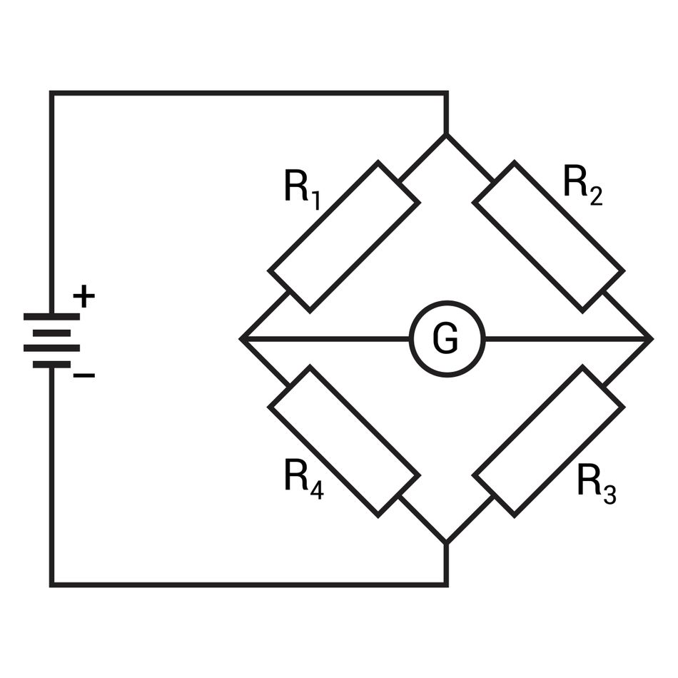
The Wheatstone bridge is a resistive network composed of four arms arranged in a diamond, forming a fundamental electric circuit governed by Ohm's Law, where current flows through each arm. It is used to measure unknown electrical resistances. Two resistors R1 and R2 form one voltage divider, and two resistors R3 and R4 form the second. These dividers share a common excitation voltage Vexc, but their junctions (VSIG+ and VSIG-) are measured differentially. A galvanometer or high-impedance voltmeter is connected across the midpoints of the two dividers detects any voltage difference between them. When the resistance ratios of the two dividers are equal — that is, R1/R2 = R3/R4 — the midpoint voltages are identical,no current flows through the galvanometer, and the bridge is said to be balanced. Any mismatch in the ratios deflects the galvanometer, indicating an imbalance proportional to the resistance difference.

Historical Context

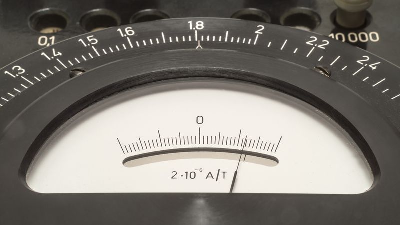
Before modern electronic instruments, the Wheatstone bridge provided a reliable method for measuring resistances. Early experimenters adjusted a known resistor until the galvanometer in the bridge read zero current, hence the term null-balance comparator. The unknown resistance could then be calculated from the known value of resistors because no current flowed through the indicator, eliminating loading errors [10]. Although the original purpose was resistance measurement, the bridge's sensitivity to small resistance changes made it ideal for strain gauges, thermistors, and other transducers.

Basic Circuit Description

The classic Wheatstone bridge configuration consists of four resistive elements arranged in a diamond and excited by a voltage Vexc. The nodes between R1 and R2 and between R3 and R4 are the differential output nodes [4]. The differential output voltage is given by:

Vdiff = (VSIG+) - (VSIG-) = Vexc(R2/(R1+R2) - R3/(R3+R4)) ... (1)

When all resistances are equal, Vdiff = 0. If one or more resistors change value (because of strain, temperature, or another stimulus), the bridge becomes unbalanced, creating an imbalance that produces a differential output proportional to the resistance change.

Wheatstone Bridge Circuit Analysis

The differential output of a Wheatstone bridge arises from the difference between two voltage dividers. Analysis of the bridge yields both balance conditions and expressions for its sensitivity.

Balanced and Unbalanced Conditions

From equation (1), balance occurs when the fraction R2/(R1+R2) equals R3/(R3+R4). Algebraic manipulation shows that the bridge is balanced when the ratio of resistances in one divider equals that in the other:

R1/R2 = R4/R3 ... (2)

When this condition holds, the output is zero, and the common-mode voltage at both output nodes equals half of the excitation voltage for symmetric resistances. If the bridge contains active sensor elements, ambient conditions (such as temperature) that change all resistances equally will preserve the balance and thus cancel out common-mode effects [1]. For example, connecting two identical strain gauges in opposite arms of the bridge compensates for uniform temperature changes because both gauges experience the same resistance drift [1].

Differential Voltage Expression

When the bridge is unbalanced, equation (1) produces a differential voltage that depends on the ratio of resistances. In a general case with one variable resistor Rx = R + ΔR and three fixed resistors equal to R, the differential output is:

Vout = (Vexc/2)(ΔR /(2R + ΔR )) ... (3)

For small changes, ΔR << R, the denominator approximates 2R and the output becomes linear: Vout ~ (Vexc/(4R)) * deltaR. This is the characteristic transfer function of a quarter-bridge sensor. As ΔR grows larger, nonlinearity increases because the denominator increases; this effect limits the usable range of a quarter-bridge measurement.

If two resistors change by equal and opposite increments (half-bridge configuration), the differential output doubles because the numerator becomes 2*ΔR  and the denominator remains similar. With four equal active resistors (full bridge), the output becomes:

Vout = Vexc * (deltaR/R) ... (4)

which is linear over a wide range [4]. These derivations will be revisited when comparing quarter-, half-, and full-bridge configurations.

Bridge Sensitivity and Nonlinearity

Bridge sensitivity refers to the ratio of output voltage change per unit fractional change in resistance (ΔR/R). For a quarter-bridge with one active resistor, sensitivity is roughly Vexc/(4R). In a half-bridge, sensitivity doubles; in a full bridge, sensitivity quadruples. This scaling is crucial because sensor outputs are often microvolt-level; more active elements yield higher signal amplitude and better immunity to common-mode effects. Nonlinearity is strongest in quarter-bridges due to the nonlinear denominator in equation (3). In high-precision applications, designers typically restrict ΔR/R to well below 1% to maintain acceptable linearity, though the exact threshold depends on the application.

Wheatstone Bridge Formula and Derivation

While equation (1) provides the general differential output, the bridge balance equation (2) and simplified forms for common configurations are invaluable in instrumentation design. This section derives these formulas and explores their implications.

Deriving the Balance Equation

Starting from the node-voltage expression of a general Wheatstone bridge, the voltage at the positive output node is:

VSIG+ = Vexc(R2/(R1+R2)) and VSIG- = Vexc (R3/(R3+R4))

The differential output is their difference. Setting this difference to zero and rearranging terms yields equation (2), R1/R2 = R4/R3. The product form R1R3 = R2R4 is also common and underlines the notion that the bridge is balanced when the product of opposite arms is equal. In a null-measurement system, the unknown resistor, Rx is placed in one arm, and the other resistors are adjusted until Vdiff = 0; then Rx = (R2/R1)*R3 [10].

Sensitivity Derivation for Common Configurations

Consider a bridge with excitation voltage Vexc, baseline resistance R, and fractional change δ = ΔR/R.

• Quarter-bridge: Vout ≈ (Vexc/4)·δ. For Vexc = 5 V, gauge factor k = 2, and 500 µε applied strain, δ = 1×10⁻³ and Vout ≈ 1.25 mV.

• Half-bridge: Vout ≈ (Vexc/2)·δ. Sensitivity doubles and the ΔR-dependent nonlinearity of equation (3) is eliminated [4].

• Full-bridge: Vout = Vexc·δ. Sensitivity is four times that of the quarter-bridge and the response is linear for all values of δ [4].

These expressions reveal the trade-off between the number of active elements and sensor wiring complexity. Full-bridge circuits provide the highest sensitivity and best linearity at the cost of additional strain gauges and wiring, whereas quarter-bridges are simple but produce smaller, nonlinear outputs.

Types of Wheatstone Bridge Configurations

Depending on the number and arrangement of active sensing elements, Wheatstone bridge circuits can be classified into quarter-bridge, half-bridge, and full-bridge configurations. Each has variations (Type I, Type II, etc.) depending on whether the sensing elements measure axial or bending strain and whether compensating gauges are used [8].

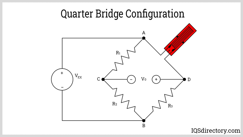
Quarter-bridge

A quarter-bridge has one active element and three completion resistors. It is the simplest configuration, requiring only one bonded gauge and two or three wires, depending on whether a three-wire lead compensation technique is used. Quarter-bridge type I measures axial strain; type II measures bending strain and uses a dummy gauge for temperature compensation. Because only one resistor changes, the bridge output follows equation (3) and its linearization in equation (4). The sensitivity at 1000 microstrain is around 0.5 mV/V for typical metal strain gauges [8]. Quarter-bridges are cost-effective and easy to install, but are susceptible to temperature-induced resistance changes unless a dummy gauge is used in an adjacent arm. Lead-wire compensation is often achieved through three-wire techniques.

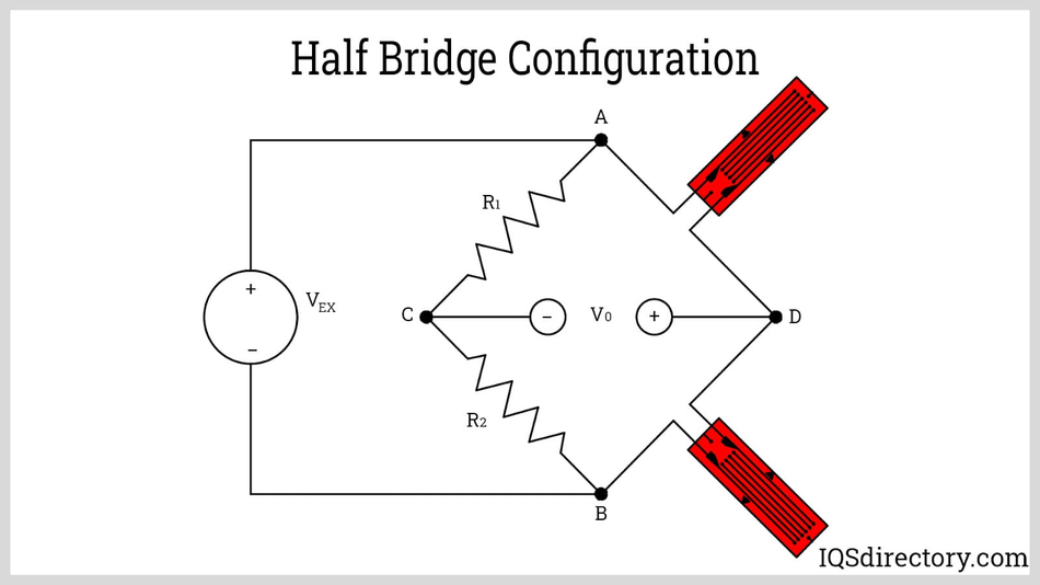
Half Bridge

A half-bridge uses two active elements. In Type I, both gauges are bonded to the specimen but oriented such that one measures tensile strain and the other compensates for Poisson's effect; in Type II, the gauges measure bending strain on opposite sides of a beam. Half-bridges require two completion resistors and three wires. Because two resistors change by equal and opposite amounts, sensitivity doubles relative to a quarter bridge [4]. The sensitivity at 1000 microstrain ranges from approximately 0.65 mV/V to 1.0 mV/V, depending on the arrangement [8]. Temperature effects partially cancel because both active gauges experience the same ambient conditions.

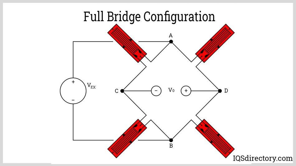
Full bridge

A full-bridge has four active gauges and no completion resistors. Type I uses four axially oriented gauges — two in tension and two in compression — for axial load measurement with Poisson compensation. Type II is configured for bending, with two gauges on the tension face and two on the compression face. Type III is adapted for torsion or shear, with all four gauges oriented at ±45° to the principal stress axis. Full-bridges require four gauges and four signal wires but no completion resistors. They offer the highest sensitivity (approximately 2.0 mV/V at 1000 µε for a gauge factor of 2) and the best common-mode rejection [8]. Because all four gauges change, temperature and lead-wire effects largely cancel. A full bridge is ideal for load cells and precision force transducers, but requires access to multiple faces of the structure and involves greater wiring complexity.

Comparison of Bridge Configurations

Wheatstone Bridge Strain Gauge Applications

Strain Gauge Fundamentals

A strain gauge is a resistive element that changes resistance when stretched or compressed. The gauge factor k defines the sensitivity and is approximately 2 for metallic foil gauges [2]. The relative change in resistance is related to strain by:

ΔR/R₀ = k · ε or ε = (1/k)(ΔR/R₀) ... (6)

For example, a 500 microstrain produces a 0.1 % change in resistance of a 120 ohm gauge. Strain gauges may be bonded to a structure with adhesive and oriented along or perpendicular to the expected strain direction. When excited with a voltage, their resistance change can be detected using a Wheatstone bridge.

Tension Versus Compression

When a structure is stretched (tension), the strain gauge elongates, increasing its resistance; compression shortens the gauge, decreasing its resistance. A quarter-bridge senses only one direction at a time; half-bridge and full-bridge configurations can arrange gauges such that one experiences tension and another experiences compression. This arrangement doubles or quadruples the differential output because one gauge's resistance increases while the other decreases [4]. Gauges oriented transversely can compensate for Poisson's ratio; e.g., in a half-bridge type I, the second gauge is aligned perpendicular to the primary gauge exploit transverse strain caused by the Poisson effect, where ν is typically 0.28–0.30 for steel. Note that this arrangement increases sensitivity by a factor of (1+ν) rather than fully doubling it.

Strain Measurement Process

Bridge completion: For quarter and half bridges, resistors known as bridge completion resistors are used to complete the bridge. These resistors must closely match the nominal gauge resistance (e.g., 120 ohm, 350 ohms, or 1 kohm) because mismatches cause offset errors. National Instruments notes that nominal gauge resistances are commonly 120 ohm, 350 ohm and 1000 ohm; choosing a higher resistance reduces power dissipation and minimizes lead-wire errors [8].

Excitation: Apply a DC excitation voltage, typically 3 V to 10 V. Higher excitation increases sensitivity but also increases self-heating; choose the highest voltage that does not cause temperature drift beyond acceptable limits. Some applications use current excitation to improve nonlinearity or AC excitation to reject thermoelectric offsets [7]. AC excitation alternates the excitation polarity, averaging out DC offsets [7].

Signal conditioning: Because the bridge produces only millivolt-level signals, an instrumentation amplifier amplifies the differential output. The amplifier should provide a high common-mode rejection ratio (CMRR), low input offset and drift, and high input impedance to avoid loading the bridge [12]. Amplifier gain is chosen based on the desired output voltage or ADC input range. For example, in a load-cell transmitter design, the differential voltage changes by about 95 microvolts per pound of load; the instrumentation amplifier gain must be roughly 2100 V/V to produce a 0.5 V to 4.5 V output range [5].

Calibration: Bridge circuits require offset and gain calibration. Zero-balance (no load) offsets due to resistor tolerances are measured and subtracted; gain calibration ensures that a known strain corresponds to the expected output voltage. Full-bridge sensors often include built-in shunt resistors for calibration.

Temperature and Lead-wire Compensation

Resistance changes due to temperature can masquerade as strain (a phenomenon known as apparent strain). Manufacturers minimize temperature sensitivity by selecting gauge alloys with low temperature coefficients of resistance; however, residual effects remain. Using a half-bridge or full-bridge with active gauges cancels common-mode temperature changes because all gauges experience the same temperature [8]. Dummy gauges — gauges bonded to an unstrained but thermally identical part of the specimen — are also used for compensation in quarter-bridge configurations.

Lead wires add resistance that changes with temperature. Two-wire connections add the full lead resistance to the gauge measurement, causing significant errors when lead resistance exceeds approximately 0.1% of the gauge resistance [11]. Three-wire connections cancel most of the lead resistance error by routing a third wire back along the same cable, allowing the measurement circuit to subtract the lead drop; four-wire Kelvin connections remove lead resistance entirely and are common in precision load cells. Shielding and twisting the leads reduces electromagnetic interference [11].

Wheatstone Bridge in Sensor Systems

While strain measurement is the most common application of Wheatstone bridges, the topology also benefits other sensors. This section surveys common sensors that employ bridge circuits.

Load Cells and Force Sensors

Load cells convert force into strain using a mechanical structure instrumented with strain gauges. Most load cells use a full-bridge configuration to maximize sensitivity and linearity. Typical sensitivity is about 2 mV/V, meaning that at 10 V excitation, the differential output is only 20 mV [6]. Precision instrumentation amplifiers are therefore necessary to amplify the signal. Because all gauges in a load cell change equally with temperature, the full bridge inherently compensates for temperature. Some load-cell circuits convert the amplified bridge output into a 4-20 mA current loop for industrial environments; Texas Instruments' reference design shows how a 1 kohm bridge with current-limiting resistors and a discrete two-amp instrumentation amplifier can achieve +/-0.1 % accuracy [5].

Pressure Sensors and Piezoresistive Bridges

Many pressure sensors use piezoresistive diaphragms in which the stress-induced resistance changes of four implanted or diffused resistors form a Wheatstone bridge. Applied pressure deforms the diaphragm, changing the resistance. Full-bridge topologies provide high sensitivity and good temperature compensation. Silicon piezoresistive sensors may integrate the bridge on the chip to minimize lead-wire errors and improve matching. Sensitivities vary widely (e.g., 10 mV/V to 100 mV/V) depending on the diaphragm geometry.

Strain-Gauge-Based Torque and Bending Sensors

Torque transducers often use full bridges with gauges at 45-degree angles to capture shear strain; bending sensors may use half bridges to measure tension on one side and compression on the opposite side. In bending beams, Type II half-bridge configurations mount two gauges on opposite sides to measure bending strain only [8]. This arrangement doubles sensitivity and cancels axial strain.

Temperature Sensors

Resistance temperature detectors (RTDs) and thermistors can also be measured using Wheatstone bridges. For example, a Pt1000 RTD (1000 ohm at 0 degrees C) in a bridge yields a differential voltage of 577 microvolts when the temperature increases by 0.2 degrees C, and the bridge is excited by a suitable voltage [9]. Bridge measurement reduces the required ADC resolution because the output is proportional to the fractional change in resistance rather than the full resistance. However, modern high-resolution ADCs often allow direct ratiometric measurement of RTDs without a bridge. NTC thermistors placed in one arm of a bridge can be intentionally unbalanced to measure temperature over a limited range; proper resistor selection removes the mean DC offset and linearizes the output [10].

Recommended Reading: RTD vs Thermocouple: A Comprehensive Guide for Engineers

Signal Conditioning for Wheatstone Bridge Outputs

Instrumentation Amplifiers

Wheatstone bridge outputs are typically in the microvolt to millivolt range, so precision amplification is essential. A difference amplifier using a single operational amplifier suffers from loading because its input impedance is limited by the feedback network. Instrumentation amplifiers (INAs) overcome this limitation by using a three-op-amp topology to achieve high input impedance, excellent common-mode rejection, and programmable gain. Analog Devices notes that INAs can deliver common-mode rejection ratios exceeding 100 dB and maintain microvolt-level offset voltages [12]. High common-mode rejection is crucial when the bridge output is only tens of millivolts but sits on top of several volts of common-mode excitation.

EDN magazine emphasises that instrumentation amplifiers, not difference amplifiers, should be used for bridge sensors. Their high input impedance prevents bridge loading, and adjustable gain sets the output swing within the subsequent ADC's range [7]. Amplifiers should also feature low 1/f noise because bridge sensors operate at low frequencies, often below 1 kHz, where 1/f noise dominates over broadband thermal noise [5].

Ratiometric ADC Interfacing

Ratiometric measurement is a common technique for digitizing bridge outputs. The principle is to use the same voltage source for both bridge excitation and ADC reference. As a result,e the ADC output code becomes proportional to Vin/Vref, so any variation in excitation voltage cancels out [4]. This approach reduces accuracy requirements on the excitation source; variations due to supply noise or temperature drift affect both numerator and denominator equally. High-resolution delta-sigma ADCs with differential inputs and programmable gain amplify the bridge signal and deliver digital output directly.

Current-Loop Interfaces

In industrial environments, 4-20 mA current loops transmit sensor signals over long distances with high immunity to noise. A common architecture is to amplify the bridge differential voltage using an instrumentation amplifier and then convert the voltage to a current with a current-loop transmitter such as the XTR116. Texas Instruments' reference design shows that for a 1 kohm bridge and 4.096 V excitation, adding 500 ohm current-limiting resistors reduces the bridge current to 2 mA and sets the effective excitation voltage to 2.096 V [5]. The instrumentation amplifier provides gain (here approximately 2100 V/V) to map the bridge's 95 microvolt/lb sensitivity to a 0.5 V to 4.5 V range [5]. The amplifier's output drives the current transmitter, which scales 0.5 V to 4.5 V to 4 mA to 20 mA for transmission. Low-drift, zero-offset amplifiers such as the OPAx387 family provide microvolt offset and low 1/f noise, making them well suited for this signal chain [5].

Excitation Source Selection

Selecting the excitation source influences bridge sensitivity, power dissipation, and measurement noise. Higher excitation voltages produce larger output signals but cause self-heating in strain gauges, RTDs, and other resistive sensors, which introduces apparent strain or temperature errors. Current excitation can reduce the nonlinearity of a single-element quarter-bridge by approximately half [4] but may complicate calibration because the bridge output voltage then depends on the source impedance. AC excitation eliminates DC offsets caused by thermoelectric voltages by reversing the excitation polarity periodically [7]; the bridge output is then synchronously demodulated to recover the measurement signal. Regardless of excitation method, the supply must be low-noise and well-decoupled at the bridge terminals; some instrumentation amplifiers include an integrated reference pin to set the output midpoint voltage and minimize common-mode range issues [5].

Recommended Reading: Difference Amplifier: Theory, Design, and Applications for Engineers

Practical Design Considerations

Designing a Wheatstone bridge measurement system involves more than selecting gauges and amplifiers. Several practical factors influence accuracy and reliability.

Gauge and Completion Resistor Selection

Strain gauge selection begins with three parameters: nominal resistance, gauge factor, and self-temperature compensation (STC) code. Common nominal resistances are 120 Ω, 350 Ω and 1000 Ω. Higher resistance gauges dissipate less power for a given excitation voltage, reducing self-heating errors. The STC code should match the thermal expansion coefficient of the substrate material — a mismatch produces apparent strain under zero mechanical load.

Completion resistors should match the nominal gauge resistance to within ±0.1% and have a TCR below 10 ppm/°C. For critical applications, bulk-metal-foil resistors offer TCRs below 2 ppm/°C and superior long-term stability.

Excitation Voltage and Self-Heating

Excitation voltage directly sets bridge sensitivity, but also sets power dissipation in every bridge arm. The maximum allowable excitation is constrained by self-heating, which shifts the gauge temperature independently of mechanical strain, introducing drift indistinguishable from the real signal. A practical guideline is to limit gauge dissipation to the manufacturer's recommended level, typically 25–100 mW, depending on gauge size and substrate thermal conductivity. In battery-powered or high-channel systems, where average power must be minimized, pulsed excitation applies Vexc only during the ADC conversion window, preserving full output amplitude while reducing thermal load.

PCB Layout and Grounding

Locate the instrumentation amplifier as close as possible to the bridge connector to minimize the length of high-impedance differential traces. Route the excitation supply and signal return on separate traces to avoid resistive coupling between the high-current excitation path and the microvolt-level signal path. Use a solid ground plane beneath the analog signal path and avoid routing digital clock lines parallel to bridge signal traces. Place bypass capacitors directly at the instrumentation amplifier supply pins. If the bridge and amplifier are on separate boards, connect the cable shield to analog ground at the amplifier end only to prevent ground loops.

Mechanical Installation

Gauge bonding quality is frequently the limiting factor in a strain measurement system. Bond the gauge to a clean, lightly abraded surface using an appropriate adhesive — cyanoacrylate for general-purpose work, epoxy for elevated temperature or long-term installations. After bonding, verify insulation resistance between the gauge grid and substrate; values below 100 MΩ indicate moisture ingress or adhesive contamination and will cause offset drift. Gauge orientation should align with the principal strain axis to within ±2° to keep cosine alignment error below 0.1%.

Calibration

A complete calibration addresses three error sources: offset, gain, and nonlinearity. Offset calibration measures the bridge output under zero stimulus and stores the value for subtraction. Gain calibration applies a known reference stimulus and adjusts amplifier gain or a digital scale factor accordingly. Where physical loading is impractical, shunt calibration places a precision resistor across one bridge arm to simulate a known resistance change, verifying the complete signal chain without mechanically loading the structure. For quarter-bridge circuits, a software nonlinearity correction using the known ΔR/R relationship from equation (3) can reduce nonlinearity error by an order of magnitude.

Common Errors and Troubleshooting

Despite careful design, Wheatstone bridge systems may exhibit unexpected behaviour. The following issues are common:

• Unbalanced output with no load: Causes include mismatched completion resistors, variations in gauge resistance, lead-wire resistance, and solder-joint resistance. Check the nominal values of all resistors and verify that the gauge is not strained by installation stresses. Use a dummy gauge or resistor network to adjust the balance and apply bridge offset compensation in the instrumentation amplifier.

• Saturation of instrumentation amplifier: The common-mode voltage at the amplifier inputs may exceed the allowable range when the bridge is excited by a single supply. To maximize input headroom, set the bridge common-mode voltage near mid-supply using a reference buffer circuit [7]. Alternatively, use a rail-to-rail instrumentation amplifier and ensure that the excitation and gain settings do not drive the output to the supply rails.

• Noise and interference: If the output contains 50 Hz or 60 Hz hum or high-frequency noise, inspect cable routing and shielding. Keep bridge leads away from power lines and motors; twist and shield them, and use low-pass filters. Verify that the instrumentation amplifier's power supply is properly decoupled with bypass capacitors.

• Nonlinear response: A quarter-bridge output becomes nonlinear at large strain because the denominator in equation (3) changes appreciably. Limit the maximum expected strain or use half-bridge or full-bridge configurations. Nonlinearity can also result from adhesive creep or material yielding; ensure that the specimen operates within its elastic range and that the gauge adhesive is rated for the operating temperature and strain level.

• Temperature drift: If the output changes with ambient temperature, ensure that temperature compensation is implemented using dummy gauges or full-bridge configurations. Check for self-heating due to excessive excitation and verify the TCR of completion resistors against the gauge alloy specification, and confirm that the STC code of the gauge matches the substrate material.

• Lead-wire errors: Excessive lead resistance may cause gain errors. Use three- or four-wire Kelvin connections and ensure that sense lines are connected directly at the gauge terminals, not at an intermediate connector or junction box. For long cables, use shielded twisted pairs and measure the lead resistance separately to apply correction.

Systematic troubleshooting involves isolating each component (gauge, wiring, amplifier, and ADC) and verifying its behaviour against design expectations.

Conclusion

The Wheatstone bridge remains a cornerstone of precision measurement. Its ability to convert tiny resistance changes into differential voltages, cancel common-mode effects, and support ratiometric measurement makes it indispensable for load cells, pressure sensors, strain gauges, and temperature sensors. Understanding the bridge equations, choosing the appropriate configuration (quarter, half, or full), and carefully designing the excitation and signal-conditioning circuitry are essential to obtain accurate results. 

Modern instrumentation amplifiers with CMRR exceeding 100 dB, high-resolution delta-sigma ADCs with integrated PGAs, and 4–20 mA current-loop interfaces extend the bridge's utility into digital and industrial domains. Advances in MEMS technology have further embedded the Wheatstone bridge topology into silicon pressure and inertial sensors, where the four piezoresistive arms are diffused directly onto a micromachined diaphragm or proof mass.

At the same time, engineers must address practical realities: lead-wire resistance, self-heating, EMI, adhesive creep, gauge STC matching, and end-to-end calibration. When properly designed and implemented, a Wheatstone bridge measurement system delivers reliable, repeatable data across a wide range of industrial, aerospace, biomedical, and structural monitoring applications.

FAQs

What is a Wheatstone bridge used for?

A Wheatstone bridge measures small changes in resistance by converting them into a differential voltage. It is widely used in strain gauges, load cells, pressure sensors, RTDs, and thermistors because it provides high sensitivity, cancels common-mode effects, and supports ratiometric measurement. The bridge can also serve as a null comparator to determine unknown resistances [10].

How does a strain-gauge Wheatstone bridge work?

When a strain gauge experiences tension or compression, its resistance changes according to the gauge factor relationship ΔR/R = k·ε, where k ≈ 2 for metallic foil gauges. In a bridge, one or more gauges form the active resistive arms.  Changes in their resistance unbalance the bridge and produce a differential voltage proportional to strain. Half- and full-bridge configurations use multiple gauges oriented to measure different strain directions, providing higher sensitivity and temperature compensation [4].

How do you calculate the output voltage of a Wheatstone bridge?

The general expression for the differential output is Vdiff = Vexc(R2/(R1+R2) - R3/(R3+R4)) [4]. For a quarter-bridge with one resistor changing by ΔR, the output is Vout = (Vexc/2)(ΔR/(2R+ΔR)) [4]. In a half-bridge the sensitivity doubles; in a full bridge, the output becomes Vout = Vexc(ΔR/R) [4].

What is the difference between quarter, half, and full bridges?

The difference lies in the number of active sensing elements: a quarter bridge has one active gauge and three completion resistors; a half bridge has two active gauges and two completion resistors; a full bridge has four active gauges and no completion resistors. Sensitivity scales with the number of active gauges. Full bridges are four times more sensitive than quarter bridges [8]. Full bridges also provide superior temperature compensation and linearity, but require more gauges and wiring.

How do you compensate for temperature in a Wheatstone bridge?

Temperature changes cause resistances to drift, producing false strain signals. Compensation methods include using dummy gauges bonded to unstrained parts of the specimen (quarter bridge type II), arranging gauges in half- or full-bridge configurations so that all gauges experience the same temperature, and selecting gauges processed to match the thermal expansion of the specimen [8]. Using three- or four-wire connections also minimizes temperature-dependent lead-wire errors [11].

Why are instrumentation amplifiers necessary for bridge circuits?

Bridge outputs are often only tens of millivolts sitting on top of several volts of common-mode excitation. Instrumentation amplifiers offer high input impedance, high common-mode rejection, and adjustable gain, making them well-suited for amplifying bridge signals without loading the sensor [12]. Difference amplifiers cannot provide comparable performance and may introduce significant errors [7].

Can a Wheatstone bridge be used with current excitation or AC excitation?

Yes. Current excitation maintains a constant current through the bridge regardless of resistance changes, which can reduce nonlinearity in single-element bridges [4]. AC excitation periodically reverses the excitation polarity, cancelling thermoelectric offsets that would otherwise appear as DC drift in the output [7]; the bridge output must then be synchronously demodulated to recover the measurement signal. Both techniques are used in specialty applications but require more complex signal conditioning.

References

[1] NASA Glenn Research Center, "Wheatstone Bridge Derivations," NASA Technical Report. [Online]. Available: https://www.grc.nasa.gov

[2] K. Hoffmann, "A Practical Hint for the Application of Wheatstone Bridges," HBK (Hottinger Brüel & Kjær), Tech. Pub. [Online]. Available: https://www.hbkworld.com

[3] Analog Devices, "Sensor Signal Conditioning," Application Note AN-347. [Online]. Available: https://www.analog.com

[4] Texas Instruments, "A Basic Guide to Bridge Measurements," Application Report SLYA056A. [Online]. Available: https://www.ti.com

[5] Texas Instruments, "High-Accuracy Wheatstone Bridge to 4–20 mA Current Loop Transmitter," Reference Design TIDA-00094. [Online]. Available: https://www.ti.com

[6] Texas Instruments, "Bridge Sensor Signal Conditioning," Seminar Presentation. [Online]. Available: https://www.ti.com

[7] EDN Engineering, "Fundamentals of Bridge Measurements." [Online]. Available: https://www.edn.com

[8] National Instruments, "Measuring Strain with Strain Gages," NI Technical Documentation. [Online]. Available: https://www.ni.com

[9] All About Circuits, "RTD Measurement Using Wheatstone Bridges." [Online]. Available: https://www.allaboutcircuits.com

[10] Ametherm, "Thermistor Temperature Measurement Using a Wheatstone Bridge," Ametherm Technical Note. [Online]. Available: https://www.ametherm.com

[11] Omega Engineering, "Lead Wire Effects and Noise Reduction in Strain Gauge Measurements." [Online]. Available: https://www.omega.com

[12] Analog Devices, "Instrumentation Amplifiers," Application Note AN-43. [Online]. Available: https://www.analog.com