Machine Vision Systems: Components, AI Integration & Selection Guide

Key Takeaways

• Machine vision refers to engineered systems that illuminate, image, and process scenes in real time for visual inspection, measurement, guidance, decision-making, and identification tasks on production lines.

• Machine vision work comprises five functional blocks: illumination, imaging optics, image sensor, processing unit and the output/interface. If one block fails, it limits overall performance. So, the design starts from understanding the smallest required feature.

• Spatial resolution is governed by the Nyquist‑Shannon sampling theorem. At least two pixels must span the smallest feature of interest. For robust edge detection, three to four pixels across a defect are recommended. 

• Lighting geometry strongly affects contrast. Bright‑field front lighting highlights flat surfaces; dark‑field front lighting accentuates scratches or embossing; back‑lighting provides silhouettes for gauging; coaxial, dome, and telecentric lights handle shiny or complex surfaces.

• Real camera specifications matter. A Basler acA2440‑20gm uses a Sony IMX264 global‑shutter sensor with 2448 × 2048 pixels (5 MP), 3.45 µm pixels, 23 fps, and a GigE interface. 

• Cognex In‑Sight 9000 reaches 4096 × 3000 resolution with 3.45 µm pixels and 14 fps over 1 Gb Ethernet. Teledyne's 5GigE Genie Nano models deliver 3.2 MP at 187 fps or 12.3 MP at 49 fps. FRAMOS's IMX900 module offers 3.2 MP at 125 fps with MIPI CSI‑2 and GMSL3 interfaces.

• Since 2020, deep learning has transformed machine vision. Convolutional neural networks, transformers and anomaly‑detection models now outperform rule‑based algorithms for unstructured surfaces. 

Introduction

Machine vision refers to the engineered use of cameras, optics, lighting and computers to automatically capture and interpret images for real‑time decision‑making. It’s different from general computer vision, which pursues broad perception and research goals. Machine vision focuses on repeatable, deterministic tasks such as inspecting solder joints, measuring geometric features, reading barcodes or guiding robots. Such systems are built with industrial‑grade components, validated by standards and supported for decades. 

The field emerged in the 1980s with analog cameras and custom frame grabbers; by the 1990s, digital CCD sensors and PC‑based processing made automated inspection practical. Over the past decade, high‑resolution CMOS sensors, powerful embedded processors and sophisticated lighting have pushed the performance envelope, while the rise of deep learning after 2020 has enabled robust inspection of complex textures and unpredictable defects.

This guide discusses technical information from vendor datasheets, standards, and market reports to provide an authoritative reference for engineers. It explains the five functional blocks of a machine vision system, delves into imaging fundamentals, explores application classes, surveys real products and AI accelerators, offers selection guidance and summarizes relevant standards. 

What is Machine Vision?

Machine vision is the application of imaging and computation to derive actionable information from physical scenes. It differs from general computer vision in scope and constraints:

• Purpose: Machine vision solves specific industrial tasks with deterministic outcomes such as pass/fail decisions, measurements, etc. Computer vision includes research topics such as scene understanding, autonomous driving, and surveillance.

• Environment: Machine vision operates in controlled settings — conveyors, robotic cells, laboratory stations — where lighting, positioning and timing can be managed. Computer vision must cope with uncontrolled environments.

• Hardware integration: Machine vision systems integrate cameras, optics, illumination, processing and I/O into robust packages. They often include real‑time control outputs (e.g., digital I/O, PLC interfaces) and comply with industrial standards and safety regulations.

• Performance focus: Accuracy, throughput and reliability are paramount. Specifications like pixel resolution, frame rate, dynamic range and latency are critical, and there is less tolerance for false positives or missed detections.

Historically, early machine vision used analog cameras and discrete electronics for tasks like presence detection. Digital frame grabbers and PC‑based algorithms introduced pattern matching and edge detection. Smart cameras integrated sensor, processor and I/O into compact devices, and interface standards like Camera Link and GigE Vision simplified connectivity. 

By 2015, global‑shutter CMOS sensors offered high resolution and low noise, enabling applications from automotive paint inspection to pharmaceuticals. The next wave came around 2020, when convolutional neural networks (CNNs), transformers, and anomaly‑detection algorithms began to outperform rule‑based approaches on unstructured textures. 

Modern machine vision spreads across 2D imaging, 3D scanning, hyperspectral analysis and embedded AI inference, with systems deployed across factories, logistics centers, laboratories and farms.

Suggested Reading: A Day in the Life of a Data Annotator: Behind Computer Vision 

Functional Blocks of Machine Vision Systems

Fundamentally, a machine vision system comprises five interdependent components. Optimizing each block ensures that the system can resolve the desired features at the required throughput and accuracy. Here are the five blocks:

Illumination 

Lighting defines contrast by controlling the direction, spectrum, and uniformity of light reaching the object. Front bright‑field lighting directs light from the camera side onto the object; light reflected from flat surfaces is collected, while defects scatter light outside the lens acceptance, appearing dark. 

Dark‑field front lighting uses low‑angle ring lights so only scattered light from scratches or embossings is captured, rendering defects bright on a dark background. Back‑lighting places the light source behind the part, producing silhouettes for gauging diameters or hole positions. 

Coaxial illumination uses a beamsplitter to direct light along the optical axis, enabling inspection of highly reflective surfaces. Dome and tunnel lights provide diffuse illumination from all directions to avoid reflections on curved or highly textured surfaces. Telecentric illuminators produce collimated light, improving edge definition and depth of field for precise measurements.

Imaging Optics 

Lenses focus the illuminated scene onto the sensor. The key parameters include focal length (which determines field‑of‑view), aperture (which controls depth of field and light collection), and optical format (sensor coverage). 

Lenses come in fixed‑focal, varifocal, macro, and telecentric designs; telecentric lenses maintain constant magnification regardless of object distance and minimize perspective distortion, which is essential for accurate gauging. 

The lens's modulation transfer function (MTF) indicates how contrast varies with spatial frequency; matching lens and sensor MTF ensures that the smallest feature is resolved .

Image Sensor

Image sensor converts photons into electronic signals. Industrial cameras use CMOS or CCD sensors with global or rolling shutters. Global shutters expose all pixels simultaneously, capturing fast-moving objects without smear. Sensor characteristics include pixel size, resolution, frame rate, spectral sensitivity and dynamic range. For example:

• The Basler acA2440‑20gm camera uses a Sony IMX264 global‑shutter CMOS sensor with 2448 × 2048 pixels, 3.45 µm pixel pitch, 23 fps and GigE interface.. 

• The Cognex In‑Sight 9000 series achieves 4096 × 3000 pixels with 3.45 µm pixels, 14 fps and 1 Gb Ethernet

• Teledyne's 5GigE Genie Nano cameras provide up to 187 fps at 3.2 MP or 49 fps at 12.3 MP.

• Photoneo's MotionCam‑3D delivers 1680 × 1200 depth maps at 20 fps with 15 million points per second throughput.

Processing Unit 

The processing unit performs image acquisition, pre‑processing (filtering, alignment), feature extraction, and decision‑making. Traditional rule‑based algorithms involve thresholding, edge detection, morphology, and template matching. 

Modern systems incorporate machine learning and deep learning for classification, segmentation, and anomaly detection. Processing architectures include PC‑based systems (x86 with GPU acceleration), smart cameras (sensor plus processor), embedded platforms and field‑programmable gate arrays (FPGAs). 

• AI accelerators like NVIDIA Jetson AGX Orin deliver up to 170 sparse INT8 TOPS with 2048 CUDA cores and 12 Arm Cortex‑A78AE CPU cores. 
• Hailo‑8 provides 26 TOPS at ~2.5 W and supports multi‑stream, multi‑model inference.
• MemryX MX3 chips achieve 6 TFLOPS per chip with only 0.6–2 W consumption.
• Ambarella CVflow SoCs offer 8K video encoding/decoding and on‑chip CNN processing.

Output/ Interface 

The processed information is transmitted to downstream systems via digital I/O, fieldbus, network protocols or storage. Standardized camera interfaces simplify integration. GenICam provides a generic API and an XML descriptor, allowing any compliant camera to be controlled without vendor‑specific drivers. 

GigE Vision carries 0.96 Gbit/s over up to 100 m cables and supports PTP for nanosecond synchronization; 5GigE multiplies throughput by 5 while retaining cable length. USB3 Vision, adopted in 2013, offers 350 MB/s bandwidth and uses transport layer protocols built on USB 3.0. 

CoaXPress 2.0 combines data and power over a single coaxial cable at up to 12.5 Gbit/s per channel. MIPI CSI‑2 is ubiquitous in embedded vision modules; D‑PHY lanes support 2.5–9 Gbps per lane, and C‑PHY lanes encode 2.28 bits per symbol with up to 13.7 Gbps per lane. OPC UA provides platform‑independent, secure client‑server and publish‑subscribe communication for integrating vision systems into Industry 4.0 architectures.

Imaging Fundamentals

Spatial Resolution and Sampling

Resolving the smallest defect requires sufficient pixel sampling. According to the Nyquist‑Shannon sampling theorem, the smallest feature must span at least two pixels to be represented without aliasing. For robust edge detection, practitioners recommend three to four pixels across the defect. 

The required pixel count can be calculated from the field‑of‑view (FOV), feature size and desired pixels per feature. Let Rf be the physical size of the smallest feature, Fp the number of pixels across that feature, and FOV the width of the area imaged. The spatial resolution Rs (mm per pixel) is

Rs = Rf / Fp

The required image resolution Ri (pixels) is then Ri = FOV / Rs. For example, to detect a 0.25 mm pinhole within a 40 mm FOV with four pixels across the hole, Rs = 0.25 mm / 4 = 0.0625 mm/pixel and Ri = 40 mm / 0.0625 mm/pixel = 640 pixels.

Modulation Transfer Function

Spatial resolution alone does not guarantee contrast. The modulation transfer function (MTF) describes how contrast varies with spatial frequency, measured in line pairs per millimeter. A system's MTF is the product of the lens MTF and sensor MTF. 

The lens is limited by diffraction and optical aberrations; the smallest resolvable spot (Airy disk) has radius r = 1.22 λ f/#, where λ is the wavelength and f/# is the lens f‑number. Telecentric lenses maintain constant magnification across the depth of field, reducing measurement errors. 

Depth of Field and Focusing

Depth of field (DoF) is the axial range over which objects appear acceptably sharp. DoF increases with smaller apertures (higher f‑numbers) but reduces light throughput. Telecentric lenses and collimated telecentric illuminators can extend DoF by 20–30%. 

In systems where objects have varying heights, liquid lenses or varifocal optics enable electronic focus adjustment. Depth of focus is the tolerance in the image plane. It is critical when aligning sensors relative to the lens; sensors with larger pixels have greater depth of focus. 

For high‑speed line‑scan or time‑of‑flight systems, motion blur must also be considered; global shutters and short exposure times mitigate blur, while strobe lighting freezes fast motion.

Noise, Dynamic Range and EMVA 1288

Sensor performance is quantified by parameters defined in the EMVA 1288 standard. Release 3.1 specifies standardized measurement procedures and representation templates. The report summarises the operating point, photon‑transfer and signal‑to‑noise ratio (SNR) curves, and lists the absolute sensitivity threshold, saturation capacity, maximum SNR, and dynamic range. 

Quantum efficiency (QE) versus wavelength is optional but valuable for selecting sensors for specific lighting colors. These metrics allow objective comparison of cameras across vendors. For example, the Basler acA2440‑20gm has a quantum efficiency of 68%, a dark noise of 2.3 electrons, and a dynamic range of 73.3 dB.

Recommended Reading: The Eyes of Smart Factories - What is Machine Vision? 

Application Classes Machine Vision Systems

Machine vision applications fall into several functional classes:

Inspection

Autonomous systems check for missing components, misalignments, or surface flaws. For instance, a Cognex In‑Sight 9000 camera can inspect printed circuit boards at 14 fps over Gigabit Ethernet, while high‑speed 5GigE cameras inspect pharmaceutical blister packs at 187 fps.

Gauging and Measurement

Vision measures distances, diameters, angles and shapes. Telecentric lenses and back‑lighting provide accurate silhouettes; FRAMOS's IMX900 module captures 3.2 MP at 125 fps , suitable for measuring battery tabs on fast conveyors. 3D triangulation systems like Photoneo MotionCam‑3D achieve 15 million points/s and 40 m/s object speeds, enabling high‑throughput volume measurement.

Guidance and Robot Vision

Cameras locate workpieces and guide robots for pick‑and‑place or assembly. Vision‑guided robots in automotive plants use stereo cameras or 2D cameras with structured light to find weld points. Hand‑eye calibration and real‑time feedback minimize positioning errors.

Spectral and Hyperspectral Imaging

Beyond visible light, machine vision uses near‑infrared, short‑wave infrared (SWIR), and hyperspectral cameras to identify materials and detect contamination. These systems capture hundreds of spectral bands, requiring high throughput and advanced processing.

Suggested Reading: What Is Machine Vision And How Is It Used In Quality Control?

Industrial Applications and Use Cases

Machine vision is pervasive across industries. The table below summarizes representative cameras and sensors used in different sectors. 

Recommended Reading: Transforming Manufacturing with Machine Vision Technology 

AI and deep learning in machine vision

From Rule‑based Algorithms to Deep Learning

Traditional machine vision relies on rule‑based algorithms: thresholding, edge detection, blob analysis, pattern matching and morphological operations. These methods perform well on structured, high‑contrast scenes but struggle with variations in texture, illumination or object shape. 

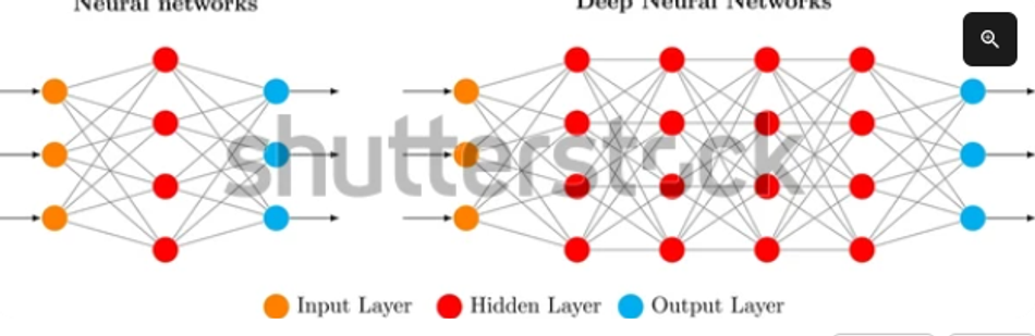
Deep learning introduced convolutional neural networks (CNNs) and, more recently, transformer architectures that learn hierarchical features directly from image data. Trained on labeled datasets, CNNs can classify defects, segment objects and detect anomalies without hand‑crafted rules. One‑class models and generative methods can identify novel defects by modeling "normal" appearance.

Transfer learning and pretrained models accelerate development, while synthetic data generation and domain randomization address the limited availability of defect samples. Transformer‑based models improve long‑range context in tasks such as text reading and irregular surface analysis.

Recommended Reading: Artificial Intelligence: A Comprehensive Guide to its Engineering Principles and Applications 

Edge AI Hardware

Deep networks require significant computation. Edge AI accelerators bring inference close to the camera, reducing latency and network bandwidth. Key platforms include:

• NVIDIA Jetson AGX Orin: Features an Ampere GPU with 2,048 CUDA cores and 64 Tensor cores, delivering up to 170 sparse TOPS of INT8 compute and 5.3 FP32 TFLOPS. The module includes a 12‑core Arm Cortex‑A78AE CPU, 32 or 64 GB LPDDR5 memory with 204.8 GB/s bandwidth, and supports up to 16 MIPI CSI‑2 lanes (40 Gbps D‑PHY or 164 Gbps C‑PHY). Power consumption ranges 15–60 W.

• Hailo‑8: A dedicated edge AI accelerator delivering 26 TOPS with on‑chip memory, enabling multi‑stream and multi‑model inference at a typical power consumption of ~2.5 W. Industrial variants operate from −40 °C to +85 °C, and automotive versions up to +105 °C.

• MemryX MX3: A neuromorphic accelerator that provides up to 6 TFLOPS per chip at 1 GHz, with an average power consumption of 0.6–2 W . Up to 16 chips can be interconnected to deliver 96 TOPS. The chip exposes a PCIe Gen3 or USB 3 interface and stores 10.5 million 8‑bit weights on‑chip.

• Ambarella CVflow SoCs: SoCs like CV7 and CV75S integrate 8K/4K video encoding/decoding and CNN acceleration with low power (under 4 W). They target robotics, drones and smart cameras with deep learning at the edge. Published marketing materials highlight 8KP60 video and CVflow architecture.

These platforms allow vision systems to run CNNs and transformers in real time, enabling complex tasks such as defect segmentation, pose estimation and cross‑modal fusion. When combined with embedded sensors and efficient protocols like MIPI CSI‑2, edge AI reduces system cost and latency.

Suggested Reading: Edge machine vision cameras powering industry innovation 

Selection For Machine Vision Systems

Choosing the right machine vision system is a multi‑factor optimization problem. Consider the following criteria:

• Inspection task and feature size: Define the smallest defect or measurement feature. Use the resolution calculation method to determine the required pixel count.

• Throughput: Calculate the required frame rate by dividing the line speed by the desired image spacing. Ensure the camera's maximum frame rate can sustain the throughput; Teledyne's 5GigE cameras deliver 187 fps at 3.2 MP for high‑speed lines, while Photoneo MotionCam‑3D captures depth maps at 20 fps with 15 million points/s for dynamic scenes.

• Lighting and environment: Choose illumination geometry that highlights relevant features (bright‑field, dark‑field, backlight, coaxial, dome or telecentric). For shiny surfaces, coaxial and dark‑field setups reduce glare. 

• Optics and sensor pairing: Match lens focal length, aperture and optical format to the sensor's pixel size and field‑of‑view. Telecentric lenses prevent perspective errors; macro lenses enable small FOVs. 

• Processing architecture: Decide between PC‑based systems, smart cameras, embedded platforms or FPGAs. Smart cameras (e.g., Cognex In‑Sight 9000) integrate sensor and processing but may limit customization. 

• Interfaces and integration: Select interfaces that support required bandwidth and cable length: GigE (0.96 Gbit/s, 100 m cables), 5GigE (5× bandwidth), USB3 Vision (350 MB/s), CoaXPress 2.0 (12.5 Gbit/s per channel), MIPI CSI‑2 for embedded modules, or GMSL3 for long‑distance coax (12 Gbps).

• Budget and scalability: Factor the cost of cameras, lenses, lighting, processing and software. Smart cameras can reduce integration effort but may be costlier per channel. 

• Build vs buy: Decide whether to build a custom vision system or purchase an off‑the‑shelf solution. Building allows optimization and cost control but demands in‑house expertise.

Standards for interoperability and safety

Machine vision operates within a framework of standards that guarantee compatibility, performance and safety.

Conclusion

Machine vision has evolved from simple binary inspection to sophisticated, AI‑driven perception. A modern system integrates carefully chosen lighting, optics, sensors, processing and interfaces. Spatial resolution and Nyquist sampling guide pixel selection; illumination geometry defines contrast; lenses and sensors must be matched via MTF; and standardized interfaces ensure integration. Deep learning and edge AI have opened new possibilities for unstructured inspection and complex tasks. 

Looking forward, machine vision will become more pervasive and intelligent. Edge AI processors will deliver teraflop‑level performance at watt‑level power, enabling real‑time 3D perception and multimodal fusion. High‑bandwidth interfaces like C‑PHY and CoaXPress 3.0 will transmit gigapixels per second. 

FAQ

1. What is machine vision?

Machine vision is the engineering discipline that uses cameras, optics, lighting and processing hardware to capture images and extract actionable information for automated decision‑making. It differs from general computer vision by focusing on deterministic industrial tasks such as inspecting, measuring, guiding or identifying objects. 

1. How does machine vision differ from computer vision?

Computer vision encompasses the broad science of enabling machines to understand images and videos, including research into perception, autonomous driving and scene understanding. Machine vision, in contrast, refers to engineered systems built for specific tasks in manufacturing and logistics. 

1. What are the components of a machine vision system?

A machine vision system comprises five functional blocks: illumination (bright‑field, dark‑field, backlight, coaxial, dome or telecentric), imaging optics (lenses that focus light and control depth of field), image sensor (CMOS or CCD camera), processing unit (PC, smart camera, embedded AI platform) and output/interface (digital I/O, Ethernet, USB, CoaXPress, MIPI CSI‑2). Standards like GenICam and GigE Vision ensure interoperability.

1. How do I choose the camera resolution?

First, identify the smallest feature you need to detect and determine how many pixels should span that feature (two pixels minimum; three to four for robust detection). Calculate the spatial resolution (feature size divided by pixels per feature) and divide the field‑of‑view by this value to obtain the required pixel count. 

1. When should I use rule‑based algorithms versus deep learning?

Rule‑based algorithms are efficient for structured problems with predictable contrast and geometry. They require engineering expertise to design filters, thresholds and feature extractors, but they run fast on low‑power hardware. Deep learning excels at unstructured tasks with variable textures, complex shapes or subtle defects. 

1. How do I select the right lighting for my application?

Assess the object's surface, geometry, and the features you need to highlight. Bright‑field front lighting illuminates flat surfaces and shows defects as dark areas. Dark‑field front lighting uses low‑angle light to emphasize scratches and embossings. 

References

1. Basler AG. acA2440‑20gm Camera Specifications and EMVA Data https://www.baslerweb.com/en/cameras/area-scan-cameras/ace/aca2440-20gm/

2. Cognex Corporation. In‑Sight 9000 Series Vision System Reference Guide https://docs.cognex.com/insight/

3. Teledyne Technologies. Genie Nano 5GigE Series https://www.teledynevisionsolutions.com/products/genie-nano-5gige/

4. Photoneo. MotionCam‑3D M+ Technical Parameters https://www.photoneo.com/products/motioncam-3d/

5. FRAMOS. IMX900 Sensor Module Datasheet https://docs.framos.com/

6. NVIDIA. Jetson AGX Orin Technical Brief https://www.nvidia.com/en-us/autonomous-machines/embedded-systems/jetson-orin/

7. Hailo. Hailo‑8 Datasheet 
   https://hailo.ai/products/ai-accelerators/hailo-8-ai-accelerator/

8. MemryX. MX3 Product Page 
   https://memryx.com/products/mx3/

9. Basler AG. GenICam Standard https://www.baslerweb.com/en/vision-campus/camera-technology/genicam/

10. Basler AG. GigE Vision https://www.baslerweb.com/en/vision-campus/interfaces-and-standards/gige-vision/

11. Basler AG. USB3 Vision https://www.baslerweb.com/en/vision-campus/interfaces-and-standards/usb3-vision/

12. Basler AG. CoaXPress 2.0 https://www.baslerweb.com/en/vision-campus/interfaces-and-standards/coaxpress/

13. Mixel. Exploring the Latest Innovations in MIPI D‑PHY and C‑PHY https://mixel.com/exploring-the-latest-innovations-in-mipi-d-phy-and-mipi-c-phy/

14. Oden Technologies. OPC UA and Industry 4.0 
    https://oden.io/

15. SICK AG. Performance Levels in Accordance with EN ISO 13849 https://www.sick.com/us/en/safety-knowledge/iso-13849/

16. Basler AG. EMVA1288 Standard https://www.baslerweb.com/en/vision-campus/imaging-basics/emva-1288/

17. Opto Engineering. Illumination Geometries and Techniques https://www.opto-e.com/basics/illumination

18. 1stVision. Imaging Basics: How to Calculate Resolution for Machine Vision https://www.1stvision.com/cameras/imaging-basics/how-to-calculate-resolution.html

19. Opto Engineering. Optimizing System Resolution: Matching Lens and Sensor MTF https://www.opto-e.com/basics/mtf