Zero Traffic Conflict (ZTC) Road Networks with Concentric Traffic Paths
U-turns and left turns are sometimes forbidden even though it increases travel distances. We demonstrate through simulations that in comparison with conventional schemes, the ZTC road network can carry approximately 50% more vehicular traffic without incurring gridlock.
This article is a part of our University Technology Exposure Program. The program aims to recognize and reward innovation from engineering students and researchers across the globe.
U-turns and left turns are sometimes forbidden even though it increases travel distances. The greater travel distances are sometimes outweighed by the improved movement through intersections due to there being fewer conflicting lanes of traffic. One can, further, forbid straight-throughs. Restricting a sufficient number of turns can make intersections free from crossing lanes of traffic (“zero traffic conflict,” “ZTC”), though there may still be merging lanes of traffic. It’s possible to make all intersections in a road network ZTC. However, keeping all destinations accessible and travel distances moderate requires careful selection of allowed driving directions and turning directions. We demonstrate through numerical microscopic and macroscopic simulations that there are road networks and ranges of traffic loads for which, in comparison with conventional schemes, ZTC road network can carry approximately 50% more vehicular traffic without incurring gridlock.
Introduction
Shorter trip lengths, other things being equal, would make for shorter trip durations, less total distances driven, less pollution, and lower costs. However, other things are not necessarily equal. If lines of traffic cross one another, one car may need to stop and wait for other cars to clear an intersection. If two lines of traffic need to merge, vehicles may need to slow down and/or take turns going into the merge lane. As a consequence, u-turns and left turns are sometimes forbidden so as to reduce conflicts. In some situations, this is worth the additional travel distances, and in some situations, it’s not worth it.
Forbidding straight-throughs is also possible, but rarely applied; even, rarely investigated. Expanding the options so as to include forbidding of straight-throughs can only improve traffic arrangements since it is a generalization of the current set of tools. There are clearly costs to forbidding straight-throughs. The benefits are still unproven.
Restricting allowed turns to the extent that there are zero-crossing lanes of traffic in the entire road network is a significantly greater restriction than in typical road networks. Keeping the average point-to-point driving distances moderate in a ZTC network requires careful choice of the allowed turns at intersections and the allowed driving directions on roads. This has been investigated in Ref. [1]. However, when a road network becomes filled with multiple vehicles, one vehicle blocks another, the simulations become nonlinear, and it becomes more challenging to determine which traffic arrangements are better and which are worse.
Road systems examined
ZTC Intersections
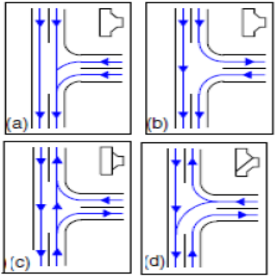
Following Ref. [1], let us review the maximum possible sets of allowed turns at intersections in which no lanes of traffic cross other lanes of traffic. We will do this for three- and four-road ZTC intersections. An intersection with one road is a dead end; an intersection with two roads is trivial; intersections of five or more roads can exist, but they are rare and their analysis is more lengthy. Three- and four-road intersections are the practically important and mathematically non-trivial cases.
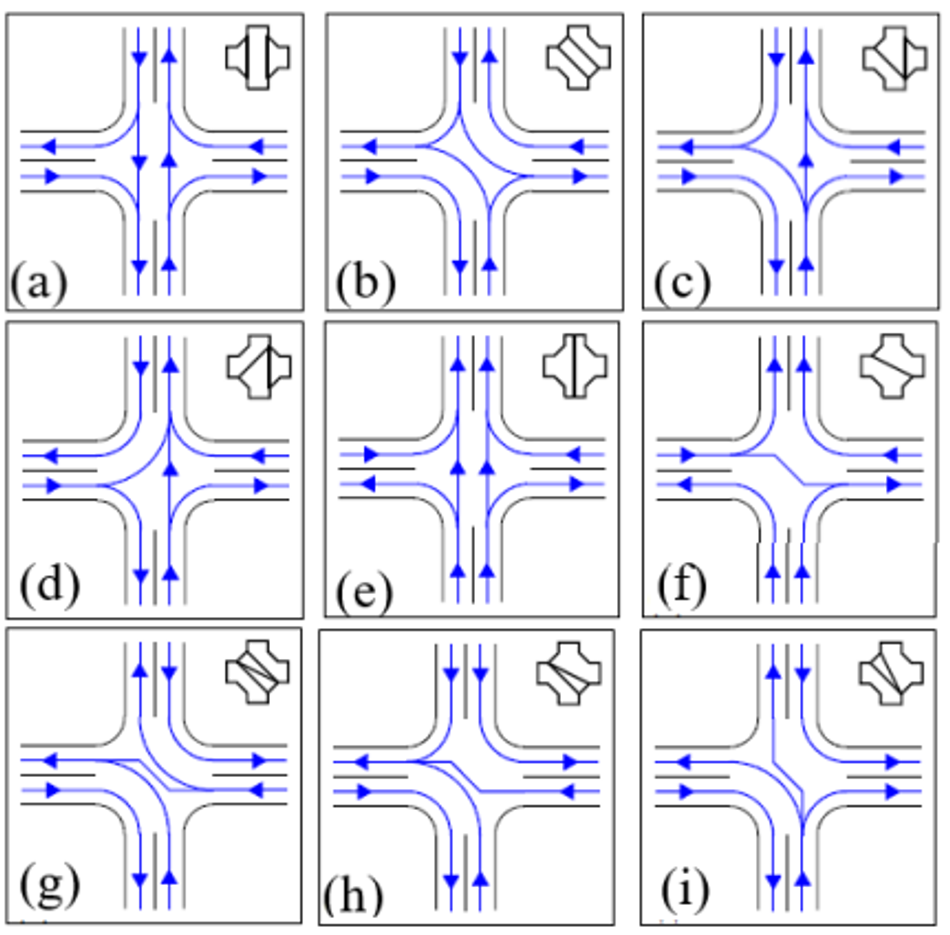
The analysis of the intersections will cover all possible combinations of one-way roads; two-way roads with right-side driving; and two-way roads with left-side driving, where within a set of codirectional lanes, driving is on the right, and large physical barriers between the mutually opposite direction lanes in a road are advisable. Figure 1 shows ZTC intersections with three roads. Figure II A shows ZTC intersections with four roads. The allowed turning directions in Figs. 1 and II A, and reflections, rotations, arrow-reversals, or deformations thereof; or one of them with some turns disallowed even though the turns are consistent with ZTC; comprise the complete set of possible ZTC intersections with three and four roads.
ZTC Road Networks
For all intersections in a road network to be ZTC, with all destinations accessible from all origins, and have the point-to-point distances only moderately longer than in road networks with unrestricted turns, the road directions and allowed turns at the intersections in the ZTC road networks need to be chosen carefully.
Reference [1] found that point-to-point driving distances could be kept within about 150% of the minimum point-to-point driving distances by having roads with allowed paths that traced concentric circles, alternating clockwise and counterclockwise. Let us examine one archetypical road network in detail: a 10x10 rectangular road network, similar to Manhattan. In Manhattan, the distance between streets averages 80.5m and the distance between avenues ranges from 186m to 280.4m. The speed limit is 25 miles per hour (= 11.2 m/s) unless otherwise posted. Until recently it was 30 MPH. On a few streets the speed limit is as high as 40 MPH. There are highways in New York City where it is 50 MPH. There are proposals to lower the default speed limit to 20 in a few neighborhoods. For this article, let’s take Manhattan but modify it so the north-south vs. east-west asymmetry is moderated and numbers are rounder. We will assume a uniform speed limit of 15 m/s, and 100m and 200m between roads. For convenience, let us take the longer sides of the blocks to be horizontal and the shorter sides of the blocks to be vertical. At the speed limit, a vehicle takes 6.7s or 13.3s to go from one intersection to the next.
In general, traffic light cycles range from 60 to 120s, and are most often in the middle of the range. For the simulations herein, we take traffic light cycles to be 90s. At that cycle duration and the chosen block lengths, vehicles driving straight can traverse several intersections with identical traffic light offsets and can expect to pass several green lights before needing to stop at a red light. We will simulate traffic lights with and without a part of the cycle reserved for pedestrians only.
Notice that that traffic light cycle is in the ballpark of an order of magnitude greater than the time for a vehicle moving at the speed limit to go from one intersection to the next. As a consequence, if one wishes to have the speed limits and traffic light periods near the convention ranges, it will only be possible to have green waves in a given direction in a route, and not in both directions.
While keeping this rectangular Manhattan-like arrangement of streets, we will simulate traffic arrangements with a variety of different intersection rules and allowed driving directions, chosen to represent a range of common intersection types. (1) One traffic arrangement that we will test is with every street two directions, right-hand driving, all turns permitted, and yield signs from all directions. We call this ”yield” or ”priority.” (2, 3, 4, 5) Another traffic arrangement that we will test is with every street two directions, right-hand driving, all turns permitted, and traffic lights at every intersection with a 90s cycle. This will be tested with all traffic lights having the same temporal offset, and with traffic lights having random offsets. We call these ”TLs” and ”randomized TLs,” with pedestrian-only crossing times and without. (6) Another traffic arrangement that we will test is with every street two directions, right-hand driving, all turns permitted, and traffic lights at every section with a 90s cycle, and the traffic light offsets staggered such that there are green waves along concentric paths, alternating clockwise and counter-clockwise. We call this ”green wave TLs.” (7) The above traffic arrangements (1–6) will be compared to the ZTC arrangement corresponding to Fig. 4 in Ref. [1], that is, with yield signs at every intersection, limitations on permitted turns so that there are no crossing lanes of traffic, some roads right-hand side driving, some roads one-way, and some roads
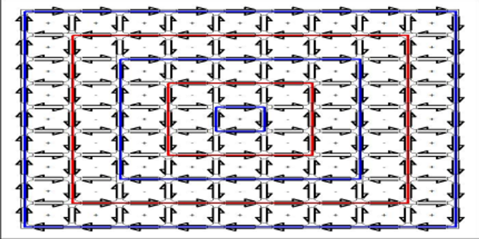
with the lanes in each direction corresponding to left-hand side driving (though right-hand side driving within each direction; this is a salient distinction only when there are two or more lanes in a given direction; in these cases, we expect there to be a barrier between the lanes in opposite directions). We call this ”ZTC.” The green-wave paths herein will correspond to the concentric clockwise and counterclockwise routes in (6), as illustrated in Fig. II B. Unlike the ZTC arrangement, which has some one-way and some left-side driving roads, the roads in the green wave arrangement simulated are all two-way and right-side driving.
Numerical Simulations
We compare the various traffic schemes – ZTC, green wave traffic lights, traffic lights with uniform offsets, traffic lights with random offsets, and with yield signs – over a range from low to very high densities. The desideratum we focus on is average trip time. We will present average trip lengths as complementary and explanatory data. Note that in other circumstances, one might be interested in optimizing other quantities, such as average fuel consumption, amount of pollution, longest travel time, average speed, average time idling, or any of various other quantities.
Simulations were carried out for streets as in Fig. II B. that is, a road network with 10x10 intersections. In one direction, the blocks are 100m apart; in the other direction the roads are 200m apart. The speed limit is 15m/s. We ran the simulations for networks with two lanes (one lane in each direction or two lanes on a one-way street) between adjacent intersections, and for four lanes (two lanes in each direction or four lanes on a one-way street) between adjacent intersections. Traffic lights have a 90s cycle.
We carried out numerical simulations of vehicles on the road networks using the software package Simulation of Urban MObility (“SUMO”), and the accompanying software package Traffic Control Interface (“TraCI”) for calling SUMO commands from within a Python program [3].
Simulations were with cars only – that is, no buses and no trains. The traffic lights in some cases included periods for pedestrian crossing, but beyond this, the individual pedestrians or bicyclists were not modeled only implicitly. Car lengths were 5m and maintained a gap of 2.5m between vehicles in front and behind. If you ignore the widths of the roads, the two-lane 10x10 rectangular road network has 54km of road lanes, and the four lane 108km. If you include the widths of the roads, you need to correct for double counting of the areas of the intersections. There are 100 intersections. The default width of the lanes in SUMO, which is what we use, is 3.2m. In reality, there will be margins beside the road and between lanes in opposite directions. For one-lane roads, there is at least 2.56km of road in the intersection; but the horizontal and vertical directions can’t be occupied simultaneously, so in effect there are 52.7km of occupiable lanes. For two-lane roads, there is a little over 10.2km of road within intersections that, although north-south and east-west moving vehicles are both permitted, they can't be occupied by cars in both directions simultaneously; that leaves 102.9km of non–double-counted road. At the car length plus the between car spacing of 7.5m, in the two-lane road case, up to 7026 cars can fit on the road network at a given time; and in the four-lane road case, up to 13720 cars can fit. Many of our simulations involve more vehicles than can fit at a given time; the starting times are spread over at least an hour, and earlier vehicles have reached their destinations before later vehicles enter the road network.
In the simulations herein, vehicles are assigned an origin, a desired start time, and a destination. The route between the start and end points are fixed at the time of departure, and are the route with the minimum predicted travel time found by a search, the traversal times on road segments based on the most recent traversal times of the road segments by other vehicles. Note that the routes are not changed during the trip. The fact that the optimum routes are calculated based on the recent travel times allows traffic to make closer to full use of the road network; it also adds nonlinearities (interactions) to the traffic dynamics. Simulations were run as ”microscopic” and as ”mesoscopic.” In SUMO’s microscopic car following model, each car bases its behavior only on the cars very close to it. In the macroscopic simulations, cars tend to fill up all lanes of the roads; and cars are permitted to turn from any lane. Closer to gridlock, the mesoscopic model seemed closer to real life; the microscopic model made vehicles more inflexible about lane choice and there were blockages that could have been avoided by vehicles being more flexible about lane choice, and in our judgment in real life this is what drivers of vehicles typically do. In real life, at higher density traffic, drivers take account of more vehicles than just the very closest ones. The resulting real-life traffic is fluid-like in ways that SUMO’s microscopic car-following and lane-changing models struggle to duplicate. It’s possibly merely accidental that So, paradoxically, the mesoscopic model appeared to give more realistic results than the microscopic model at high density cars beyond the ones immediately ahead of and beside them and they make an effort to move as far forward as they can, which more fluid-like than the microscopic algorithm is able to represent.
In the simulations, cars are scheduled to depart at even intervals in the first hour. The departure points and the arrival points are chosen randomly. The number of cars entered into the network ranged from 1 up to approximately 80, 000, that is, from lowest density and through the point that cars experienced gridlock for hours.
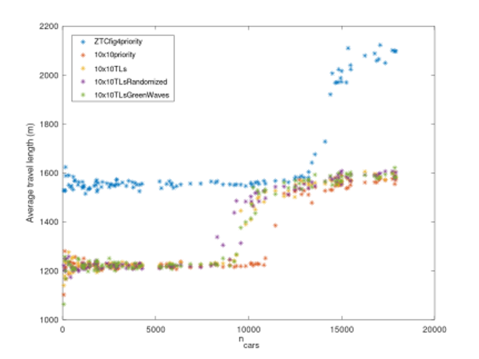
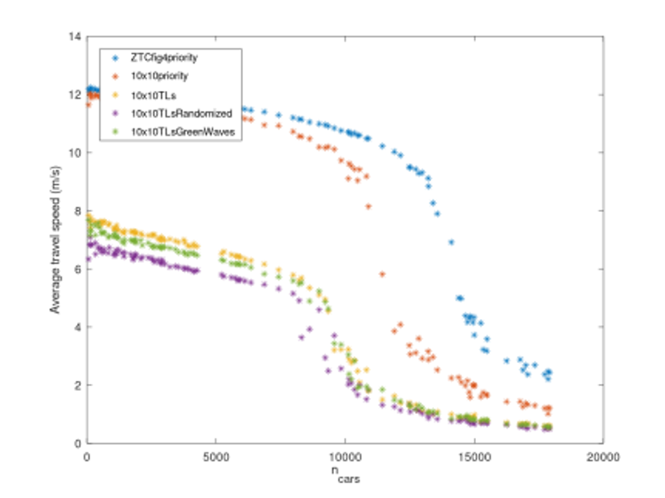
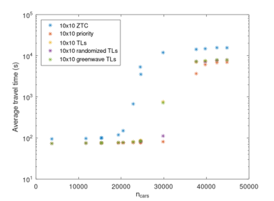
Figures 4, 5, 6 show how the different one-laned networks respond to a range of traffic loads. Figure 4 shows average trip duration, for each road network type, as a function of number of cars. Figure 5 shows average trip length, for each road network type, as a function of number of cars. Figure 6 shows average trip speed, for each road network type, as a function of the number of cars. The ZTC arrangement is worse at low traffic densities. The trip lengths are longer and there are not enough conflicts at intersections for the other types of intersection to jam up. At medium densities, the ZTC arrangement has greater throughput the intersections, and for a range of vehicle densities, this outweighs the longer trip lengths. At very high densities, the ZTC arrangement jams up also, and the advantage over other arrangements disappears. At severe gridlock, all road networks performed approximately equally. In this Manhattan-like road network, the ZTC allowed approximately 50% more traffic in the network before gridlock set in.
If lanes are doubled – two lanes in each direction for two-way roads and four lanes in one-way roads – drivers have the option of changing lanes. This degree of freedom can have profound effects on traffic. In some regimes, especially low traffic densities, vehicles need only be concerned with the vehicle immediately in front of them and vehicles in lanes they might turn into. On other regimes, especially high traffic densities, drivers make their decisions based on consideration of the many vehicles in their proximity. A driver might be more or less flexible about changing lanes in order to advance in heavy traffic. A driver might or might not show consideration for the needs of other drivers. Behavior might change after time elapses in the same traffic density situation because drivers may become impatient or angry. In real life, especially at high density, different populations may differ from one another in their behavior. One should not expect that there will be a universal approximately correct model for how drivers behave. In light of this, especially with multiple lanes and high densities, it makes sense to simulate traffic using various driver behavior models.
SUMO’s car-following and lane-changing models in the microscopic model have tens of adjustable parameters. Common to all SUMO’s microscopic models is that drivers take into consideration the vehicle immediately in front of them and the occupancy of adjacent lanes, but driver behavior is not directly influenced by vehicles further away. For high density traffic in networks with intersections and multiple codirectional lanes, the microscopic simulations that we observed tended to have much more blockages than in real life, apparently, due to excess driver inflexibility about changing lanes in order to advance.
Paradoxically, SUMO’s mesoscopic model, which models traffic as a flow and does not model each lane in a road separately, seemed to give dynamics closer to real life in cases where traffic is very heavy. Vehicles tended to fill up all lanes on a road. In real life, this tends to happen because drivers are aware of the wider traffic situation and have time to plan and maneuver so as to fill most gaps. In SUMO’s mesoscopic models, this happens because vehicles fill most gaps because they are indifferent to granular details, including to granular details that a relatively simple car-following and lane-changing model are unable to capture accurately in this regime.
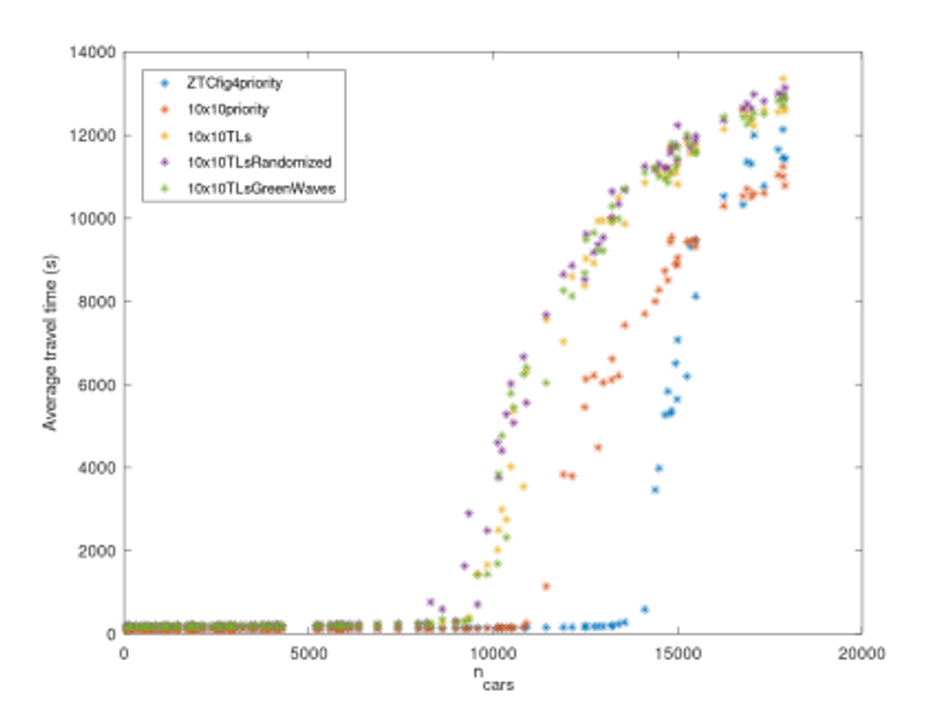
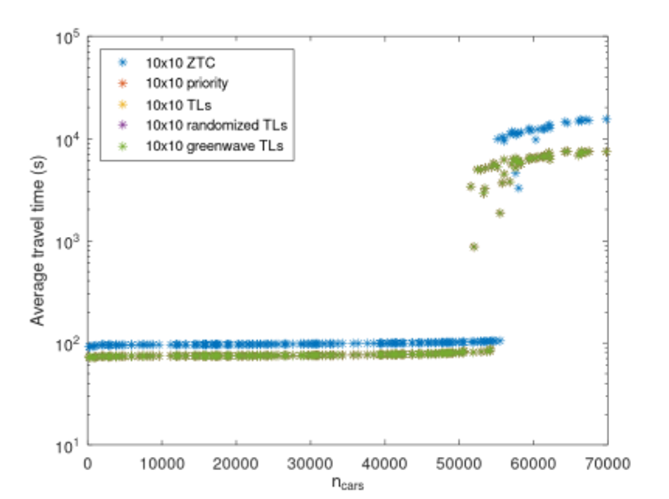
Figure 7 shows the average trip durations versus number of cars in the road network with doubled lanes, where the simulations are fully mesoscopic. Figure 8 shows the average trip durations versus number of cars in the road network with doubled lanes, where the streets are modeled in the mesoscopically, that is, as fluids, but the traffic lights are modeled as in the microscopic model. In the fully mescoscopic data, the ZTC arrangement has the longest travel times for low traffic densities. As the traffic density increases, all the non-ZTC traffic arrangements show instability about when they reach gridlock; in some cases the ZTC will slightly underperform the non-ZTC arrangements, as at low densities, but sometimes the non-ZTC arrangements will hit gridlock, while the ZTC does not, and ZTC often strongly outperforms the non-ZTC schemes. There is a very small range of densities at which the non-ZTC arrangements consistently reach gridlock but ZTC does not. Past that point, both ZTC and non-ZTC reach gridlock, and ZTC moderately underperforms ZTC. In the partially mesoscopic simulations, the ZTC arrangement always has the longest travel durations.
Discussion and conclusions
We showed that at moderately heavy traffic loads, a zero-traffic conflict (ZTC) arrangement with concentric alternating direction paths can be optimal for an archetypical road network arrangement, a 10x10 Manhattan-like rectangular network. For a network of one-lane roads, where modeling driver behavior is relatively straightforward, we found that with the ZTC arrangement, the road network can accommodate significantly more traffic than traffic lights or yield signs with all turning directions permitted. That is, in the ZTC arrangement that keeps added distances moderate, gridlock does not set in until a volume of cars that is about 50% greater than the volume at which gridlock sets in for a variety of standard traffic arrangements for the same road network.
The cost of the ZTC arrangement is approximately 30% longer travel durations and trip lengths when the traffic density is low. For a network of two lane roads, we found that average trip durations were highly sensitive to how driver behavior is modeled. In the real world, driver behavior is not constant or universal. We modeled driver behavior microscopically (every vehicle and every lane distinctly modeled), mesoscopically (more fluid-like), and a mix of the two. The microscopic-model behavior at high traffic densities did not seem realistic at all, we believe because drivers there only take into account vehicles immediately ahead and of the occupancy of adjacent lanes. The mesoscopic and partly-mesoscopic models both appeared plausible, even though they differed from one another. In these simulations, there were sometimes ranges near the gridlock threshold in which the ZTC arrangement outperformed conventional traffic arrangements. The sensitivity to driver behavior in simulations and in real life implies that there is potential for ZTC arrangements to improve the carrying capacity of road networks, but one must be careful to implement it where and when it can do the most good and not where the effect of longer travel distances will outweigh the benefits.
The road networks tested were small enough for the entire network to have approximately the same traffic conditions everywhere. In a larger and more heterogeneous road network, such as a whole city, there are likely to be areas of high traffic density and also areas of low traffic density. One could ask how the advantages and disadvantages of ZTC arrangements balance out, and also if there are ways to adjust so that the advantages of ZTC arrangements are maximized and the disadvantages of ZTC arrangements are minimized.
References
[1] D. Eichler, H. Bar-Gera, and M. Blachman, “Vortex-Based Zero-Conflict Design of Urban Road Networks,” Netw. Spat. Econ. 13, 229-254 (2013). doi:10.1007/s11067-012-9179-x
[2] S. D. Boyles, T. Rambha, and C. Xie, “Equilibrium Analysis of Low-Conflict Network Designs,” Transportation Research Record: Journal of the Transportation Research Board 2467, 129–139 (2014). DOI: 10.3141/2467-14 Transportation Research Board of the National Academies, Washington, D.C.,
[3] P. A. Lopez et al., “Microscopic Traffic Simulation using SUMO”; IEEE Intelligent Transportation Systems Conference (ITSC), 2018.
[4] Tasgal, R.; Eichler, D. Zero Traffic Conflict (ZTC) Road Networks with Concentric Traffic Paths. Preprints 2021, 2021110223 (doi: 10.20944/preprints202111.0223.v1).
About the University Technology Exposure Program 2022
Wevolver, in partnership with Mouser Electronics and Ansys, is excited to announce the launch of the University Technology Exposure Program 2022. The program aims to recognize and reward innovation from engineering students and researchers across the globe. Learn more about the program here.