Dynamic simulation and optimization of anaerobic digestion processes using MATLAB

This article is a part of our University Technology Exposure Program. The program aims to recognize and reward innovation from engineering students and researchers across the globe.

Time series-based modeling provides a fundamental understanding of process fluctuations in an anaerobic digestion process. However, such models are scarce in literature. In this work, a dynamic model was developed based on modified Hill’s model using MATLAB, which can predict biomethane production with time series. This model can predict the biomethane production for both batch and continuous process, across substrates and at diverse conditions such as total solids, loading rate, and days of operation. The deviation between literature and the developed model was less than ± 7.6%, which shows the accuracy and robustness of this model. Moreover, statistical analysis showed there was no significant difference between literature and simulation, verifying the null hypothesis. Finding a steady and optimized loading rate was necessary to an industrial perspective, which usually requires extensive experimental data. With the developed model, a stable and optimal methane yield generating loading rate could be identified at minimal input. 

Introduction

Anaerobic Digestion (AD) is an established technology which con-verts organics to energy (CH4) and biofertilizer. However, there are several consortia of microbes and process parameters involved in this conversion, which makes it difficult to achieve an optimum yield. Pro- cess stability and optimization could be achieved through process con- trol strategies such as models, and simulations (Kumar Khanal et al., 2021). Such strategies play a pivotal role in understanding the dynamic behavior of AD and process optimization. Current mathematical models describe the AD process in a steady-state condition, where time-series prediction is scarce in literature. Moreover, such models have a defi- ciency in describing the process parameters under transient state or start-up operations resulting from changes in input. Therefore, there is a need for a dynamic model, which can predict an optimum methane yield involving process parameters yet matches with the reality. 

Dynamic models provide a reliable and efficient operation of future plants with a combination of available sensor data and laboratory analyses (Weinrich and Nelles, 2021). Andrews et.al., (1971) developed the first dynamic model for AD processes, which uses unionized acid as a rate-limiting substrate. After then, Hill and Barth, (1977) developed a model considering the inhibi- tion of fatty acids for manure and animal wastes. The cattle manure based dynamic modeling of cyclic batch reactor was developed based on kinetic constants for mesophilic conditions (Keshtkar et al., 2001). Later, IWA (International Water Association) developed the ADM1 model, that became popular and widely accepted (Batstone et al., 2006). ADM1 includes 12 algebraic and 19 differential equations with 24 dynamic variables. ADM1 describes the degradation of biochemical pathways, enzymatic hydrolysis to methanogenesis (Weinrich and Nelles, 2021). However, some processes are not included such as sulfate reduction, sulfide inhibition, and acetate oxidation reactions. Apart from ADM1, there are other models developed to predict AD processes including modified Gompertz model, simple kinetic model, empirical model (Abunde Neba et al., 2020; Karki et al., 2022; Weinrich et al., 2021). 

Anaerobic digestion is affected by several process driven factors such as loading rate (OLR), retention time (HRT), pH, temperature, and mixing (Kunatsa and Xia, 2022). These factors strongly affect methane yield. According to the author’s knowledge, time-series, or the dynamic nature of the process over an operating period with the inclusion of above-mentioned process parameters is never reported in the literature. Predicting dynamic behavior helps the industry to implement a real- time solution. 

In this work, a dynamic model was developed based on the modified Hill’s equation using MATLAB (V2021b). This is the first study to report the effect of varying loading rate with time series which works for both batch and continuous processes across range of feedstocks. The goal of this work includes: (1) develop and validate the model against literature to verify if there are any differences between them. (2) Analyze the dynamic behavior of the AD process over days of operation. (3) Study the effect of varying loading rates to find optimum methane yield over time. 

Methods

Model description

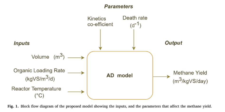
In this work, modified Hill’s model was used to (Hill and Barth,1977) forecast the dynamic behavior of the AD processes. This model used a set of differential equations characterizing the various stages of AD (hydrolysis, acidogenesis, acetogenesis, and methanogenesis). The microbial communities of various stages were divided into acid formers and methane formers. The growth rate of the microbes was modeled using Monod kinetics (Hill, 1983). The key input to the model includes organic loading rate (OLR), reactor volume, and operating temperature, while monitoring parameters included death rate and rate kinetics (Fig. 1). The model was simulated by using the MATLAB (V2021b), and the required input data such as, Monod half velocity constant, yield factors, and death rate of microbes were taken from the literature (Haugen et al., 2013; Pathmasiri et al., 2013; Saeed et al., 2019). 

Model development

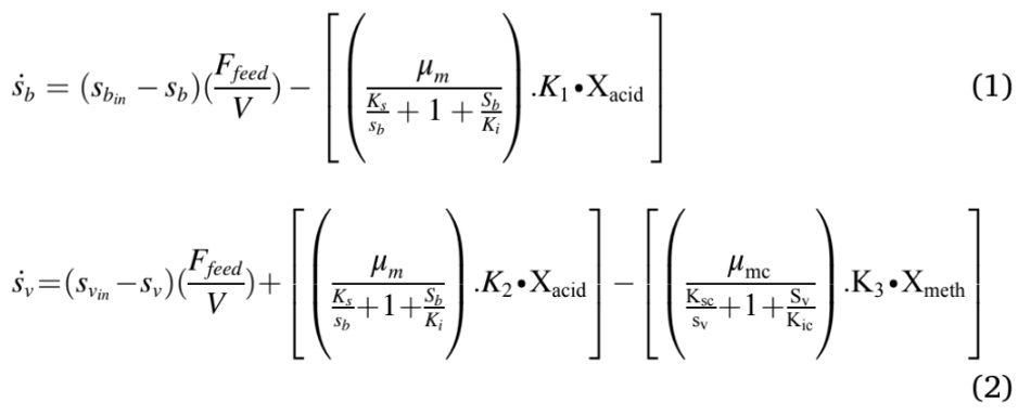
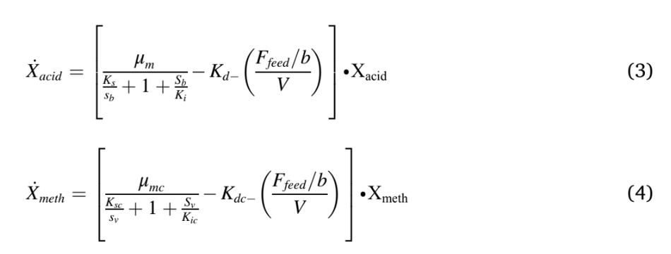
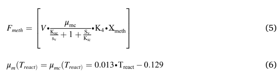
The modified Hill’s model was used in this study were described in Equations (1) to (6). Eqn. (1) & (2) was used to model the hydrolysis and acidogenesis stages of AD process. Eqn. (1) stands for the rate of change of VS breakdown in the reactor during AD processes. The change in VS concentration was found by the reactor loading rate with its kinetics. The rate of change in total VFA (Volatile Fatty Acid) was obtained by adding total VFA produced with the difference between the growth rate of acid formers and methanogens (Eqn. (2)). The next stage in an AD process was acetogenesis, which figures out the rate of change in acetic acid concentration Eqn. (3). This was ob- tained by multiplying the total acid concentration with the difference between growth and death rate of acetogens, and retention time. Like Eqn. (3), Eqn. (4) stands for the rate of change of methane formation, which was obtained by multiplying the methanogens concentration with the difference between the growth and death of methanogens, and retention time. Methane volume produced from the reactor was calculated by multiplying reactor volume with the growth kinetics and concentration of methanogens (Eqn. (5)). The maximum growth rates of acidogens and methanogens were expressed in Eqn. (6), which depends on temperature. 

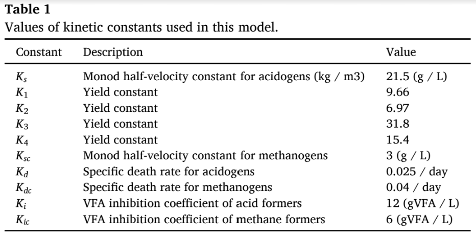
The key assumptions of this model include constant reactor stirring,reactor volume, and temperature being constant. The kinetic coefficients were obtained from (Haugen et al., 2013; Hill, 1983), while the death 

rates of acetogens and methanogens taken from the literature (Fedai- laine et al., 2015; Haugen et al., 2013; Pathmasiri et al., 2013) and the values are tabulated in Table 1. About twenty parameters were added to perform the simulations using MATLAB. These parameters include VS concentration, acid con- centration, growth rates, volume, and retention time. The equations were placed in MATLAB (Version R2021b) as main and function scripts (Anaya Menacho et al., 2022; Carlini et al., 2020). All the parameters were defined in main script, while function scripts hold the differential equations mentioned above (Eqn. (1–6)). The main script acts as an input–output model, while the function scripts perform the calculations (see e-supplementary material). The output was returned to the main scripts, from which the methane production was obtained (Weinrich and Nelles, 2021). 

Model validation

The robustness of the model was verified and validated using various literature. The variation included scale, substrate, operating parameters, and volume. Table 2 shows the operating conditions used in each sce- nario and the respective experimental yield obtained. 

Case (1): Cow manure was used as a feedstock, which was (Kaparajuet al., 2009) operated in a batch mode. The OLR was 0.328 kgVS /L with a 5-L reactor volume and the reported methane yield was 353.5 L/kgVS at a 15-day HRT. 

Case (2): This scenario used swine manure in a 30L reactor at a OLRof 7.68 gVS/m3 . The biogas obtained was 0.269 m3 /kgVS at 8 days retention time (Fujita et al., 1980). 

Case (3): Most earlier scenarios used a mono-digestion, while in this validation a co-digestion concept was assessed. The substrate composi- tion used was 70% MSW (Municipal Solid Waste) and 30% citrus waste (Forgacs ́ et al., 2012) in a 5L reactor. The methane yield reported was 0.55 m3 CH4/kgVS at 21 days HRT by using a loading rate of 3-gVS/L. 

Case (4): Food waste was used as a substrate in a continuous mode with 340 m3 reactor volume. The methane yield reported was 0.59 m3 CH4/kgVS at 48 days HRT with a OLR was 6.4 kgVS/m3 /d.(Liu et al., 2020). 

Case (5): MSW was used as a substrate in a continuous mode (Eliyanet al., 2007). This was a pilot reactor with a volume of 600L operating at a OLR of 3 gVS/L/d with 19 days HRT. The reported biogas production was 401 L/kgVS. 

Case (6): This scenario used an industrial data using MSW, with a volume of 3000-m3, running at a OLR of 3.5 kgVS/m3 /d. The biogas production from that plant was 9600 m3 /d at 21 days HRT (Rajendran et al., 2014). 

Statistical analysis

The scenarios that were confirmed against the model was evaluated for its significance through statistical analysis. A probability plot was drawn for the difference between the experimental results reported and simulated results obtained. Key statistical indicators such as P-value, mean, and standard deviations were looked out for. This probability plot used a 95% confidence interval. Minitab (V19) was used to plot the probability plot. 

Sensitivity analysis

The key inputs to the model were the loading rate and solids con-centration. The sensitivity of the model to the solid’s concentration was evaluated by varying it in a range of ± 5%, ±10%, ±20%. A trend line was plotted across these variations and the resulting R2 value was re- ported, and it was checked for correlation. 

Loading rate optimization

The modified Hill’s model predicts the biomethane production,however the loading rate at which maximum yield obtained was not embedded. The OLR was optimized in MATLAB using the interior-point algorithm and minimum constraint solver (fmincon) (Khan et al., 2016) (Donoso-Bravo et al., 2011). The solver works based on lower- and upper- bound limits in an iterative process. The iteration was repeated until maximum methane yield and the respective loading rate was re- ported as output. 

Results and discussion

The Modified Hill’s model was applied in this study, while examining diverse operating conditions of AD. The simulations could predict the methane yield across substrates, loading rates, and temperature in a dynamic timeframe with an accuracy of 92 ± 7.6%. The simulation was confirmed with literature ranging from laboratory to industrial data, and the differences were calculated. Besides, statistical analyses and sensi- tivity of the model was assessed to prove its robustness. 

Model validation

The operating conditions, experimental yield, simulation yield and the difference between the two for various case studies were summa- rized in Table 2. The difference between simulation and experimental methane yield varied between + 7.5 to − 7.6%. For instance, scenario-2 used a swine manure which was run in a batch mode had reported an experimental biogas yield of 0.266 m3 /kgVS, while the dynamic model developed in this study reported the biogas yield of 0.269 m3 /kgVS. The error difference between the simulation and experimental yield was − 1.1%. This error difference could be due to lack of ammonia inhibition (Lee et al., 2018). The variation of simulation and experiments were dependent on the assumptions, inhibition, and equation considered in this study. This work had considered VFA inhibitions whereas other inhibitions such as ammonia were not considered due to lack of exper- imental data. Hence, the variation of results varied between ± 7.6%. The inhibition rate of each feedstock is different while we used an in- hibition data from (Haugen et al., 2013; Hill, 1983), which may lead to a deviation from the experimental values reported. 

Fig. 2 shows the dynamic response from the model alongside experimental and simulated values. The batch process had a fixed amount of VS available and hence over the higher days of operation, the substrate gets degraded which was reflected as the decrease in the bio- methane/biogas yield Fig. 2(a-c). In addition, In Fig. 2(c) the experi- mental yield reported was 0.555 m3 CH4/kgVS, while the simulation reported a yield of 0.621 m3 CH4/kgVS at 21 days HRT. However, the dynamic response from the simulation shows that at 10 days HRT, 0.692 m3 CH4/kgVS could be achieved. This shows that the reactor was not operated at maximum biomethane yield. As the VS decreases, the biomethane / biogas yield decreases over time in a batch process (Fig. 2 a-c). Contrastingly, in continuous pro- cesses (Fig. 2 d-f), the biogas/methane yield did not decrease, instead a steady state condition was achieved. This was due to the continuous supply of VS in these processes (Fig. 2d-f). Fig. 2(d) shows that the difference between experimental and simulated result was 0.3% at 48 days retention time. Nonetheless, running the reactor at 30 days reten- tion time did not decrease the methane yield by greater than 5%. 

Such a trade-off could be predicted from the simulation which can help the industry or research community for a better decision making and operation of the digester. This trade-off offers a 37% reduction in reactor volume, without compromising on the methane yield significantly. Various models have been developed in the past that has predicted the AD processes for batch, and continuous operations. ADM1 was widely accepted by academia and industry as it was a comprehensive model accounting for most of the factors that affect the biomethane production (Donoso-Bravo et al., 2011). Most models work either for a batch or continuous process, and only a few of them could predict both the processes (Westerholm et al., 2020). The model developed in this work was one such, which can predict both batch and continuous pro- cesses. For a batch process, degradation rate over time was a critical parameter, while for a continuous process, achieving a steady-state condition influences the importance. 

The current model we had developed could maximize the loading rate and methane yield. However, certain shortcomings need to be addressed. This includes the effect of mixing such as agitation speed, and duration that might affect the methane yield in industrial applications. Besides, this model considered only volatile fatty acids inhibition, while other inhibitions such as ammonia, metal ions, and foaming were not included. Including them in further versions of the model will enhance the robustness and accuracy in implications of it. Furthermore, we considered the solids loading, C/N ratio, while adding the composition of substrate as carbohydrates, proteins and fats will help in having a deeper understanding in model prediction.. This model had an accuracy of 92%, while similar models in the literature reported an accuracy varied between 80 and 97% (Anaya Menacho et al., 2022; Rajendran et al., 2014). The sample size used to validate the work was a critical parameter, as it will accounts for vari- ation in operating conditions, feedstock etc. In this work, six different cases were considered, while several literatures had limited sample size comparison (three or less). A robust and reproducible model needs validation across various data; shortcomings such as inputs hinders developing full-proof models. 

Statistical analysis

Evaluating the simulation statistically shows the accuracy of its robustness. A statistical analysis was conducted to check the significance of difference between random scenarios mentioned earlier and their error difference between experimental and simulated results. The probability plot was drawn to check the P-value and the significance of differences with a 95% confidence interval (CI) for various scenarios (Fig. 3). The P-value obtained was 0.377 (greater than0.05), shows that across random scenarios the difference between experimental and simulated results were insignificant, which verifies the null hypothesis(Hamawand and Baillie, 2015; Rajendran et al., 2014; Silva and De Bortoli, 2020). Null hypothesis tests the statistical significance between two data sets verifying if there were any difference between observed and measured values (in this case literature and model). Null hypothesis assumes that the population were randomly distributed with equal variance. 

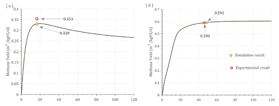
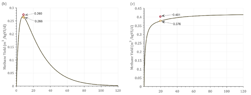
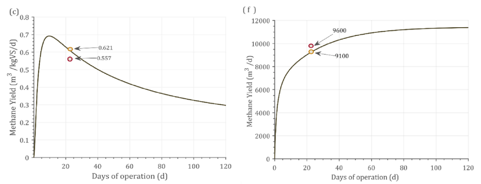
Fig. 2. Dynamic response of the model against experimental results. (a) Cow manure (TS 6%), (b) Swine manure (TS 6.4%), (c)MSW + CW (TS 13%), (d) Food waste (TS 32%), (e) MSW (TS 10%), (f) MSW (TS 15%).

In literature, only a few had statistically validated between experi-mental and simulated data. Few reasons could be the smaller sample size, and lack of input data from experiments. For instance, Anaya Menacho et al. (2022) developed a model to predict AD processes using Aspen Plus with a sample size of 3 data points; however, it was not statistically validated. Zhu et.al (2019) used modified Gompertz model in a batch process to study of effect of methane production from dead and sick pigs. Statistical analysis showed no significant difference be- tween the two models on the predicted biomethane production. Like this study, Rajendran et.al (2014) reported the P value was 0.701, showing no significant difference between literature and experiments. However, it was a steady-state model, whereas in this study, dynamic time-series based prediction of methane production was carried out. 

Sensitivity analysis

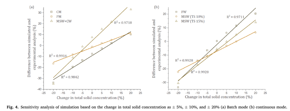
Sensitivity analysis shows the effect of critical parameters on the model output and its efficacy. The critical input to the model is TS (Total Solid) concentration (Calise et al., 2020), which was altered by ± 5%, ±10%, and ± 20% for both batch and continuous processes to study its sensitivity. Fig. 4 shows the effect of sensitivity analysis for batch (a) and continuous processes (b). Both batch and continuous processes showed a linear correlation with varying solids concentration. This correlation explains the strength of relationships between the total solid concen- tration and the difference between experiment and simulated data. 

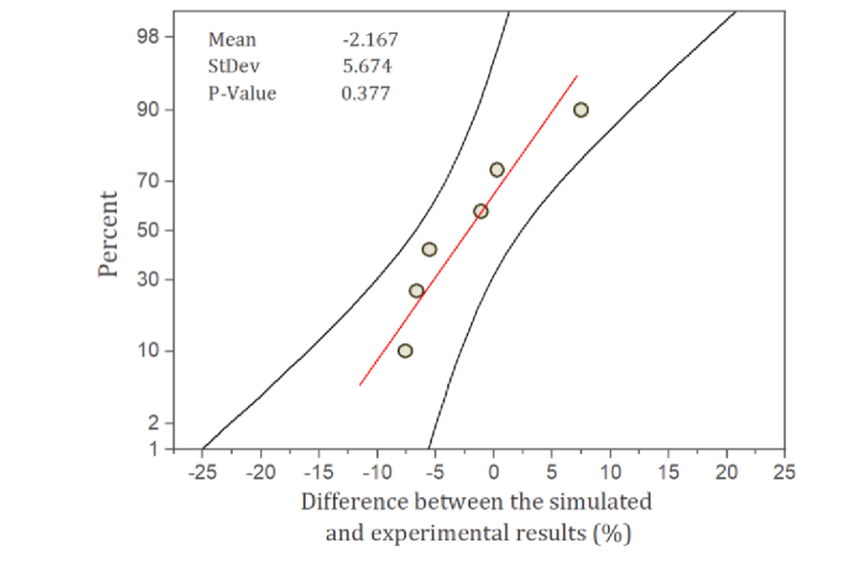
Fig. 3. Probability plot of the different cases validated against the simulated result.

The average R2 value was 0.98, and 0.986 for batch and continuous pro- cesses, respectively. Higher the variation of solid concentration deviates the accuracy of difference between experimental and simulated data. This shows that accurate TS was needed to predict the model. However, the linear correlation can help to identify the proximity of the bio- methane estimation. The change in the TS concentration will have a deviation in prediction from the original simulated data. This deviation was linear meaning that any such change from an application perspec- tive could be predicted for linearity and correlation. This strong corre- lation shows the higher degree of robustness and accuracy of the model. A study by Mukumba et al., (2018), showed a similar correlation against the experimental data and the R2 value was 0.97. 

Effect of methane production on various loading rates

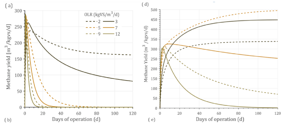
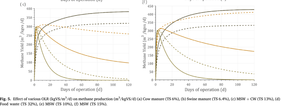
Optimizing the OLR for a given substrate improves productivity and methane yield. An attempt was made to optimize OLR by simulating the experimental data against certain standard conditions including 500-m3 reactor volume and 37 ◦C as operating temperature. Under these con- ditions, the optimal loading rate at which maximum methane yield obtained was identified. Optimizing the OLR against standard condi- tions reduces any errors within the operating parameters. Different OLRs were simulated for optimization including 2,3,5,7,9, and 12 kgVS/m3 / day. The type of feedstock, composition, and its operating conditions have a varying optimal point on OLR. For example, food waste (Fig. 5d) had an optimal OLR of 5 kgVS/m3 /day, while MSW (Fig. 5f) had an optimal OLR of 3 kgVS/m3 /day. 

This could be explained by the fact that food waste has easily degradable organics, while MSW was a complex sub- strate and hence higher loading could not be achieved. Until 20 days of operation (Fig. 5f), OLR of 2 kgVS/m3 /day received a maximum methane yield, while after that 3 kgVS/m3 /day had a higher methane yield. This shows that longer days of operation could optimize better loading rates, or which helps in reaching a steady-state condition. In Fig. 4(e), OLR of 3 kgVS/m3 /day could not support its stability, while 2 kgVS/m3 /day could maintain steady state at a longer operating period. Such time-dependent predictive analytics were not reported in literature elsewhere, shows the importance, innovation, application, and usability of such simulation in industries. Eliyan et al. (2007) reported that increasing the OLR from 2 to 2.5 kgVS/m3 /d using MSW as a substrate saw a decline in methane yield from 140 to 62.5 m3 CH4/kgVS/d (55.3%). The same study when simulated with the current model by increasing the OLR from 2 to 2.5 kgVS/m3 /d revealed a methane yield decline from 108 to 66.6 m3 CH4/ kgVS/d (38.2%) depicting the reality shows the reproducibility of the model and its validation against experimental data (Fig. 5e). 

Optimization studies

Optimizing the loading rate through experiment was not easy, as multiple trials were necessary. Upon analyzing the various models re- ported in the literature showed the following findings: 1. Several works have a smaller sample size, which leads to reduced precision and ac- curacy. However, the major issue in such smaller size was the lack of consistent data availability in literature. 2. A sizeable number of models have included time series, while optimizing them over process param- eters were not considered. In this work, optimization based on loading rate over time was illustrated. However, with a standard input given and by using the optimization algorithm in MATLAB, the maximum methane of an AD process could be predicted. Lower loading rates yield low methane, while higher loading creates imbalance and decreases the stability (Khan et al., 2016). Hence, running at the optimum point is essential for maximum profitability. 

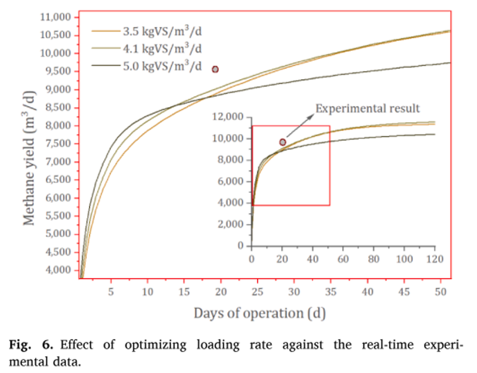
As different studies reported distinct inputs and combinations, a standard condition was assumed to evaluate the maximum loading rate prediction. This includes a reactor size of 3000-m3 running at mesophilic temperature (37 ◦C). Experimental data of case-6 reported operating at 3.5 kgVS/m3 /d, and the methane yield was 9600 m3 /d. Increasing the loading rate to 5.0 kgVS/m3 /d in simulations showed a decline in methane yield to 8600 m3 /d (Note: The errors between simulation and experiments are not considered here) (Fig. 6). A lower and upper bound limit was given to the optimization algorithm in MATLAB based on the flow rate, which in term governs the loading rate, solid concentration. 

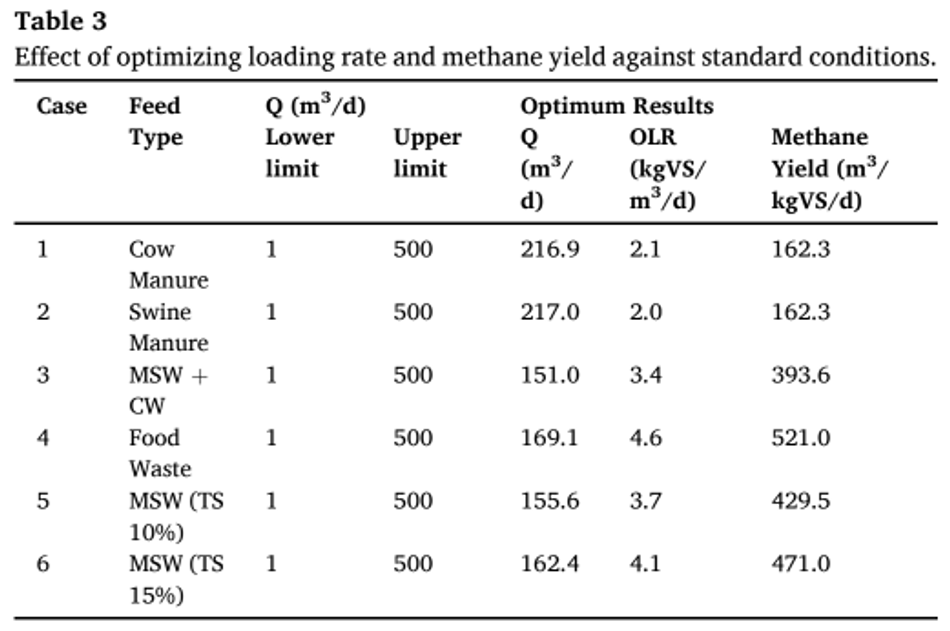
The lower bound flow rate was kept at 1-m3 /d, while the upper bound value was kept at 500-m3 /d. The output from MATLAB yielded an optimum OLR of 4.1 kgVS/m3 / d against the experimental data of 3.5 kgVS/m3 /d. Adding the error difference from base case (-5.5%) scenario; the simulation resulted in a methane yield of 9875 m3 /d (OLR- 4.1 kgVS/m3 /d) against 9600 m3 / d from experiments (OLR- 3.5 kgVS/m3 /d). Similarly, each base case was optimized to find its maximum loading rate and methane yield, that was reported in Table 3. The optimum conditions obtained for food waste (case (4), according to simulations reached an OLR of 4.6 kgVS/ m3 /d with a methane yield of 521 m3 /kgVS/d. Similarly, case (3) using MSW with citrus waste reported a maximum loading of 3 kgVS/m3 /d, while simulation optimized the loading rate to 3.4 kgVS/m3 /d.

Conclusion

In this work, time-series based modeling was developed predicting the dynamic behaviour of AD using MATLAB. The model had an accu- racy of 92 ± 7.6% across variety of feedstocks and processing condi- tions. This model could be applied to batch and continuous processes, which was rare in literature. The loading rate was optimized to yield maximum methane production, that also showed the region of stability from an operational perspective. The implications of this work include to use it real-time operations of an AD plant and laboratories to estimate the best region of operation in terms of loading rate and yield.

CRediT authorship contribution statement

Prabakaran Ganeshan: Methodology, Formal analysis, Visualiza-tion, Writing – original draft, Software, Validation. Karthik Rajendran: Conceptualization, Investigation, Supervision, Writing – review & edit- ing, Project administration. Acknowledgments Prabakaran Ganeshan acknowledges the University Research Fellowship (URF) received from SRM University-AP to conduct this work. 

Supplementary data

Supplementary data to this article can be found online at https://doi.org/10.1016/j.biortech.2022.126970.

References

1. Abunde Neba, F., Asiedu, N.Y., Morken, J., Addo, A., Seidu, R., 2020. A novel simulation model, BK_BiogaSim for design of onsite anaerobic digesters using two-stage biochemical kinetics: Co Digestion of blackwater and organic waste. Sci. African 7, e00233. https://doi.org/10.1016/j.sciaf.2019.e00233. 

2. Anaya Menacho, W., Mazid, A.M., Das, N., 2022. Modelling and analysis for biogas production process simulation of food waste using Aspen Plus. Fuel 309, 122058. https://doi.org/10.1016/j.fuel.2021.122058. 

3. Batstone, D.J., Keller, J., Steyer, J.P., 2006. A review of ADM1 extensions, applications, and analysis: 2002–2005. Water Sci. Technol. 54, 1–10. https://doi.org/10.2166/ wst.2006.520. 

4. Calise, F., Cappiello, F.L., Dentice d’Accadia, M., Infante, A., Vicidomini, M., 2020. Modeling of the anaerobic digestion of organic wastes: Integration of heat transfer and biochemical aspects. Energies 13 (11), 2702. 

5. Carlini, M., Castellucci, S., Mennuni, A., Selli, S., 2020. Simulation of anaerobic digestion processes: Validation of a novel software tool ADM1-based with AQUASIM. Energy Reports 6, 102–115. https://doi.org/10.1016/j.egyr.2020.08.030. 

6. Donoso-Bravo, A., Mailier, J., Martin, C., Rodríguez, J., Aceves-Lara, C.A., Wouwer, A.V., 2011. Model selection, identification and validation in anaerobic digestion: A review. Water Res. 45, 5347–5364. https://doi.org/10.1016/j.watres.2011.08.059. 

7. Eliyan, C., Adhikari, R., Juanga, J.P., Visvanathan, C., 2007. Anaerobic Digestion of Municipal Solid Waste in Thermophillic Continuous Operation. Int. Conf. Sustain. Solid Waste Manag. Asian Inst. Technol, Thail https://doi.org/10.1.1.539.3346. 

8. Fedailaine, M., Moussi, K., Khitous, M., Abada, S., Saber, M., Tirichine, N., 2015. Modeling of the anaerobic digestion of organic waste for biogas production. Procedia Comput. Sci. 52, 730–737. https://doi.org/10.1016/j.procs.2015.05.086. 

9. Forgacs,  ́ G., Pourbafrani, M., Niklasson, C., Taherzadeh, M.J., Hov ́ ath, I.S., 2012. Methane production from citrus wastes: Process development and cost estimation. J. Chem. Technol. Biotechnol. 87, 250–255. https://doi.org/10.1002/jctb.2707. 

10. Fujita, M., Scharer, J.M., Moo-Young, M., 1980. Effect of corn stover addition on the anaerobic digestion of swine manure. Agric. Wastes 2, 177–184. https://doi.org/ 10.1016/0141-4607(80)90014-1. 

11. Hamawand, I., Baillie, C., 2015. Anaerobic digestion and biogas potential: Simulation of lab and industrial-scale processes. Energies 8, 454–474. https://doi.org/10.3390/ en8010454. 

12. Haugen, F., Bakke, R., Lie, B., 2013. Adapting dynamic mathematical models to a pilot anaerobic digestion reactor. Model. Identif. Control 34, 35–54. https://doi.org/ 10.4173/mic.2013.2.1. 

13. Hill, D.T., 1983. Simplified monod kinetics of methane fermentation of animal wastes. Agric. Wastes 5, 1–16. https://doi.org/10.1016/0141-4607(83)90009-4. 

14. Hill, D.T., Barth, C.L., 1977. A Dynamic Model for Simulation of Animal Waste Digestion All use subject to JSTOR Terms and Conditions A dynamic of animal model waste for simulation digestion. Water Pollut. Control Fed. 49, 2129–2143. 

15. Kaparaju, P., Ellegaard, L., Angelidaki, I., 2009. Optimisation of biogas production from manure through serial digestion: Lab-scale and pilot-scale studies. Bioresour. Technol. 100, 701–709. https://doi.org/10.1016/j.biortech.2008.07.023. 

16. Karki, R., Chuenchart, W., Surendra, K.C., Sung, S., Raskin, L., Khanal, S.K., 2022. Anaerobic co-digestion of various organic wastes: Kinetic modeling and synergistic impact evaluation. Bioresour. Technol. 343, 126063 https://doi.org/10.1016/j. biortech.2021.126063. 

17. Keshtkar, A., Ghaforian, H., Abolhamd, G., Meyssami, B., 2001. Dynamic simulation of cyclic batch anaerobic digestion of cattle manure. Bioresour. Technol. 80, 9–17. https://doi.org/10.1016/S0960-8524(01)00071-2. 

18. Khan, M.A., Ngo, H.H., Guo, W.S., Liu, Y., Nghiem, L.D., Hai, F.I., Deng, L.J., Wang, J., Wu, Y., 2016. Optimization of process parameters for production of volatile fatty acid, biohydrogen and methane from anaerobic digestion. Bioresource Technology 219, 738–748. 

19. Kumar Khanal, S., Lü, F., Wong, J.W.C., Wu, D.i., Oechsner, H., 2021. Anaerobic digestion beyond biogas. Bioresour. Technol. 337, 125378. Kunatsa, T., Xia, X., 2022. A review on anaerobic digestion with focus on the role of biomass co-digestion, modelling and optimisation on biogas production and enhancement. Bioresour. Technol. 344, 126311 https://doi.org/10.1016/j. biortech.2021.126311. 

20. Lee, D.J., Bae, J.S., Seo, D.C., 2018. Potential of biogas production from swine manure in South Korea. Appl Biol Chem 61 (5), 557–565. Liu, Y., Huang, T., Li, X., Huang, J., Peng, D., Maurer, C., Kranert, M., 2020. Experiments and modeling for flexible biogas production by co-digestion of food waste and sewage sludge. Energies 13 (4), 818. 

21. Mukumba, P., Makaka, G., Mamphweli, S., 2018. Mathematical modelling of the performance of a biogas digester fed with substrates at different mixing ratios. Asian J. Sci. Res. 11, 256–266. https://doi.org/10.3923/ajsr.2018.256.266. 

22. Pathmasiri, T.K.K.S., Haugen, F., Gunawardena, S.H.P., 2013. Simulation of a Biogas Reactor for Dairy Manure Simulation of a Biogas Reactor for Dairy Manure 394–398. 

23. Rajendran, K., Kankanala, H.R., Lundin, M., Taherzadeh, M.J., 2014. A novel process simulation model (PSM) for anaerobic digestion using Aspen Plus. Bioresour. Technol. 168, 7–13. https://doi.org/10.1016/j.biortech.2014.01.051. 

24. Saeed, M., Fawzy, S., El-Saadawi, M., 2019. Modeling and simulation of biogas-fueled power system. Int. J. Green Energy 16, 125–151. https://doi.org/10.1080/ 15435075.2018.1549997. 

25. Silva, M.I., De Bortoli, A.L., 2020. Sensitivity Analysis for Verification of an Anaerobic Digestion Model. Int. J. Appl. Comput. Math. 6, 1–12. https://doi.org/10.1007/ s40819-020-0791-z. 

26. Weinrich, S., Mauky, E., Schmidt, T., Krebs, C., Liebetrau, J., Nelles, M., 2021. Systematic simplification of the Anaerobic Digestion Model No. 1 (ADM1) – Laboratory experiments and model application. Bioresource Technology 333, 125104. 

27. Weinrich, S., Nelles, M., 2021. Systematic simplification of the Anaerobic Digestion Model No. 1 (ADM1) – Model development and stoichiometric analysis. Bioresource Technology 333, 125124. 

28. Westerholm, M., Liu, T., Schnürer, A., 2020. Comparative study of industrial-scale high- solid biogas production from food waste: Process operation and microbiology.  Bioresour. Technol. 304, 122981 https://doi.org/10.1016/j.biortech.2020.122981.  

About the University Technology Exposure Program 2022

Wevolver, in partnership with Mouser Electronics and Ansys, is excited to announce the launch of the University Technology Exposure Program 2022. The program aims to recognize and reward innovation from engineering students and researchers across the globe. Learn more about the program here.